Goal
Multi-objective optimization is a problem-solving technique that involves finding the most efficient solution among several possible options that must be optimized simultaneously. For this assignment, the goal is to find an optimal maintenance strategy in order to reduce costs, system downtime, greenhouse gases, etc. Therefore, a genetic algorithm needs to be implemented in order to identify a set of Pareto-optimal solutions.
Multi-Objective Optimization
To implement a multi-objective optimization for our system, the nsga2() function, part of the mco package, was used. It was necessary to define the function to be minimized, the number of input variables, the number of output measures, and the lower and upper bounds for the input variables.
To create the function to be minimized, it is important to look at the input and output variables. For this purpose, different maintenance strategies had to be analyzed. Therefore, the durations of the interventions were considered in a specific range, as defined in the page: Maintenance Strategies.
Kindergarden interventions
- 10 ≥ M1 ≤ 20
- 3 ≥ M2 ≤ 8
- 20 ≥ M3 ≤ 35
Exterior interventions
- 12 ≥ E1 ≤ 25
- 5 ≥ E2 ≤ 10
- 27 ≥ E3 ≤ 37
An additional input variable which was varied within a range is the depth of the footing. Moreover, the output parameters for the multi-objective optimization are the total duration of the interventions, the minimum distance between two consecutive interventions, energy, CO2, NOx, SO2, and Costs.
Based on this information, it was possible to define the fitness function, which provided the following results:

Results
By using the ggplot2 package, it was possible to generate the graphs of the Pareto front. In Figure 2 the red dots form the Pareto front, which considers the total duration of the interventions and the costs of maintenance. With the help of the created Pareto front it is possible to explore the different options. The best options have a short duration of maintenance and low costs.
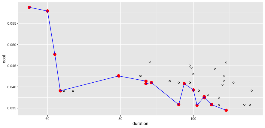
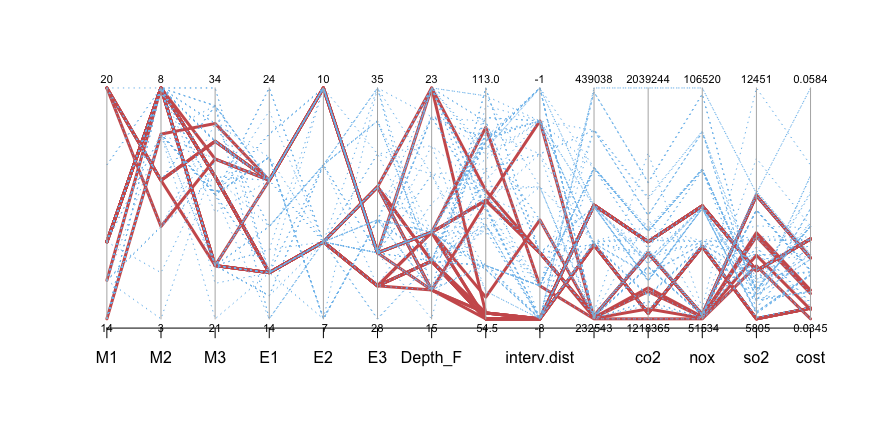
Figure 3 shows the accumulated impact of the input parameters on the performance criteria. The red lines show the solutions of the Pareto front, that are optimal. Moreover, the blue lines represent the non-optimal solutions. Overall, it can be seen that some options consume more energy or produce more greenhouse gases than others. Accordingly, depending on the scope and objective of a stakeholder, the choice of solution can vary.
← Previous Page: Life Cycle Analysis