Introduction
The infrastructure systems are aging, and their conditions are deteriorating due to factors such as usage and environmental influences. For engineering structures and systems subject to deterioration processes, commonly assumed failure scenarios involve instances where a structure weakened by deterioration suddenly experiences extreme excitation, leading to failure, or where the accumulated deterioration itself directly causes failure [1]. Effective maintenance can prolong the lifespan of components, reducing the frequency of failure events and minimizing wastage of resources on unnecessary repairs [2]. However, in many cases, both the deterioration and excitation processes are subject to significant uncertainty [1], [2]. Therefore, it is crucial to monitor the degradation process through inspections and/or automatic monitoring sensor systems. These systems can provide decision-makers with accurate assessments and prognoses of component condition states, which can then be integrated into a probabilistic framework to model the effects of degradation and the adopted maintenance policy [1], [2]. Given the importance of accurate information, it is essential that inspectors and monitoring systems collect data that can inform decision-making. This data, when integrated into decision-making processes, helps reduce uncertainty and leads to more informed maintenance actions. However, data collection is often expensive due to limited resources, necessitating prioritization. Decision-makers must balance the cost of gathering information against its potential benefits in terms of selecting more appropriate maintenance actions [2]. The planning of inspections and repair actions significantly impacts the costs associated with engineering structures or systems [1]. Therefore, it is crucial to identify optimal inspection and repair plans that minimize the total expected costs associated with inspection, repair, and failure throughout the structure’s design lifetime. This involves considering factors such as inspection methods, timing, and repair actions [1]. Once the optimal inspection and maintenance plan are identified, it is important to investigate how these plans and their associated total expected costs are influenced. Such investigations can highlight significant parameters affecting the inspection and maintenance plan and may lead to the rejection of certain plans deemed too sensitive to specific parameters [1], [2].
Integrated maintenance strategies
To integrate our diverse systems, we divided our entire system into two components: the main factory system and the railway system.
As part of our maintenance strategies, our goal is to minimize the number of intervention days throughout the system’s lifetime by introducing maintenance activities in our subsystems. To achieve this, we have focused on two distinct maintenance strategies. The first strategy includes corrective maintenance activities, while the second strategy excludes corrective maintenance and instead emphasizes preventive maintenance activities, as shown in Table 1 to Table 4. Table 1 to Table 4 give an overview of the maintenance action, their frequency, the total lifespan of the subsystem as well as their duration.
Table 1. First maintenance strategy including preventive actions for the main factory
|
Main Factory – 1st maintenance strategy |
|||||
|
Steel Purlins |
|||||
| Design Option | Event | Frequency | Total Lifespan | Duration | Maintenance action |
| 1.Hot-dip galvanized | IC | 3 | 50 | 1 | IC: Inspection and cleaning |
| 1.Hot-dip galvanized | PR | 36 | 50 | 3 | PR: Partial replacement |
| 1.Hot-dip galvanized | TR | 50 | 50 | 7 | TR: total replacement |
|
Beam and Slab |
|||||
| Design Option | Event | Frequency | Total Lifespan | Duration | Maintenance action |
| 3. beams and slabs – Reinforced Concrete with Ground granulated blast-furnace slag | S | 27 | 108 | 2 | S: Stitching |
| 3. beams and slabs – Reinforced Concrete with Ground granulated blast-furnace slag | G | 18 | 108 | 1 | G: Grouting |
| 3. beams and slabs – Reinforced Concrete with Ground granulated blast-furnace slag | RS | 36 | 108 | 3 | RS: routing and sealing |
Table 2. First maintenance strategy including preventive actions for the railway system
|
Railway System – 1st maintenance strategy |
|||||
|
Ballast Railway Track |
|||||
| Design Option | Event | Frequency | Total Lifespan | Duration | Maintenance action |
| 3.Railway Track (Concrete Sleeper with Ballast Track Bed) | M | 1 | 50 | 2 | M: Maintenance |
| 3.Railway Track (Concrete Sleeper with Ballast Track Bed) | RPR | 8 | 50 | 7 | PR: Rail Partial replacement |
| 3.Railway Track (Concrete Sleeper with Ballast Track Bed) | R | 40 | 50 | 15 | R: Replacement |
|
Foundation |
|||||
| Design Option | Event | Frequency | Total Lifespan | Duration | Maintenance action |
| 1. conventional without water – Ready mix design 1 | I | 6 | 120 | 1 | I: Inspection |
| 1. conventional without water – Ready mix design 1 | RC | 50 | 120 | 3 | RC: Recalculation |
| 1. conventional without water – Ready mix design 1 | RW | 80 | 120 | 5 | RW: Remedial work |
Table 3. Second maintenance strategy including corrective actions for the main factory
|
Main Factory – 2nd maintenance strategy |
|||||
|
Steel Purlins |
|||||
| Design Option | Event | Frequency | Total Lifespan | Duration | Maintenance action |
| 1.Hot-dip galvanized | IC | 3 | 50 | 1 | IC: Inspection and cleaning |
| 1.Hot-dip galvanized | RP | 5 | 50 | 3 | RP: Repainting |
| 1.Hot-dip galvanized | TR | 50 | 50 | 7 | TR: total replacement |
|
Beam and Slab |
|||||
| Design Option | Event | Frequency | Total Lifespan | Duration | Maintenance action |
| 3. beams and slabs – Reinforced Concrete with Ground granulated blast-furnace slag | S | 25 | 108 | 2 | S: Stitching |
| 3. beams and slabs – Reinforced Concrete with Ground granulated blast-furnace slag | G | 15 | 108 | 1 | G: Grouting |
| 3. beams and slabs – Reinforced Concrete with Ground granulated blast-furnace slag | RS | 36 | 108 | 3 | RS: routing and sealing |
Table 4. Second maintenance strategy including corrective actions for the railway system
|
Railway System – 2nd maintenance strategy |
|||||
|
Ballast Railway Track |
|||||
| Design Option | Event | Frequency | Total Lifespan | Duration | Maintenance action |
| 3.Railway Track (Concrete Sleeper with Asphalt Track Bed) | M | 1 | 50 | 2 | M: maintenance |
| 3.Railway Track (Concrete Sleeper with Asphalt Track Bed) | RPR | 10 | 50 | 7 | PR: Rail Partial replacement |
| 3.Railway Track (Concrete Sleeper with Asphalt Track Bed) | R | 40 | 50 | 15 | R: Replacement |
|
Foundation |
|||||
| Design Option | Event | Frequency | Total Lifespan | Duration | Maintenance action |
| 1. conventional without water – Ready mix design 1 | I | 6 | 120 | 1 | I: Inspection |
| 1. conventional without water – Ready mix design 1 | RC | 50 | 120 | 4 | RC: Recalculation |
Figure 1 illustrates the timeline of the integrated maintenance plan for the two subsystems utilized: the main structure, which encompasses the factory system, and the railway system.
Let’s take an example to elaborate more the difference between the 2 strategies (steel purlins):
1st Strategy
Corrective Action Strategy: This strategy targeted replacement of damaged sections of steel purlins every 36 years. Through this approach, specific areas showing signs of wear or deterioration are identified and replaced as needed, ensuring the structural integrity and longevity of the purlins.
2nd Strategy
Preventive Action Strategy: The preventive action strategy involves regular repainting of the steel purlins every 5 years. By proactively applying a protective coating, the purlins are shielded from environmental factors such as corrosion and rust, thereby excluding the need for partial replacement.
These maintenance strategies offer distinct advantages in terms of structural preservation and cost-effectiveness, providing options tailored to the specific needs and priorities of the project.
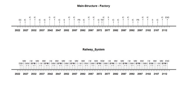
Figure 1. Timeline of the integrated maintenance plan.
As seen in Table 1 to Table 4, maintenance requirements, maintenance actions, and total lifespan exhibit significant variability. Given the diversity in maintenance actions, an effort was made to optimize the specification of individual maintenance measures with the aim of achieving higher efficiency. However, due to the inherent nature of each system, attaining such optimization proved unfeasible, leading to the adoption of two distinct maintenance strategies. The lifespan of the foundation and the beam and slab subsystems significantly exceeds that of other components due to their stringent requirements for safety, longevity, and materials usage. Assuming interconnectedness between the main factory and railway system, we project a total lifespan of 90 years for the integrated systems.
Results
Comparing the results of the two maintenance strategies, we observe that the first strategy, the preventive maintenance strategy, requires 236 days of maintenance (Figure 2), while the second, the corrective maintenance strategy, requires 231 days (Figure 3), resulting in a 6-day improvement.
Although this improvement is modest, the reduction in days implies cost savings in the second scenario.
![]()
Figure 2. Summed whole systems interventions days during the lifetime for the first maintenance strategy
![]()
Figure 3. Summed whole systems interventions days during the lifetime for the second maintenance strategy
To enhance maintenance strategies, a Pareto frontier was utilized as a tool for multi-objective optimization to determine solutions that balance multiple conflicting systems, specifically investigating criteria associated with intervention duration and intervals. Given the numerous subsystems (five in total), the parameter “n.grid” was set to two, resulting in 16,384 unique combined lifetime scenarios, as depicted in Figure 4.
![]()
Figure 4. Calculated lifetime scenarios
By running the R-Script with n.grid = 2 multiple times, it was determined that the deviation for the Pareto solutions was approximately ±10.5 for the duration and ±1 for the distance between interventions (dist.inter). Figure 5 illustrates various maintenance combinations, revealing options such as interventions with either 183 days duration and 2 years between them, or 173.5 days duration and 1 year between interventions. In either scenario, there is a compromise between duration and distance: reducing duration increases proximity, while extending the distance between interventions increases duration.
![]()
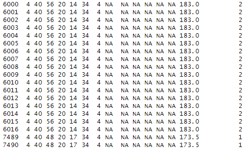
Figure 5. Best results for low(dur) and high(dist.inter) for combined lifetimes
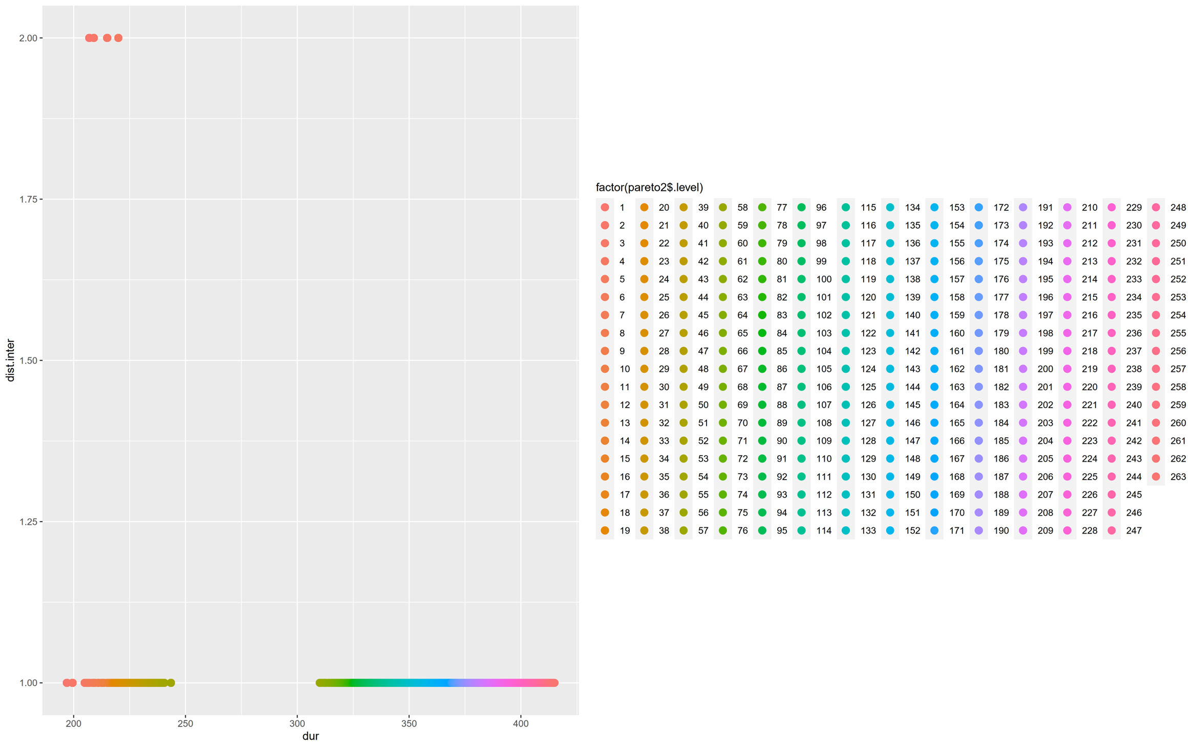
Figure 6. The pareto chart showing a set of solutions with 263 samples.
Figure 6 illustrates one set of solutions with 263 samples, representing the best trade-off between the chosen subsystems based on the preference. The plot demonstrates the relationship between the distance between interventions (dist. inter) and the duration of interventions (dur). The objective was to estimate the optimal solution, aiming for the lowest duration of overall intervention days while maximizing the number of years between interventions.
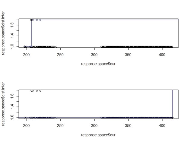
Figure 7. Evaluation of the ranking of the samples.
In Figure 7 the Pareto solutions are derived from this result set to assess the ranking of the samples. The blue lines represent the Pareto frontier, while the black dots signify the optimal combinations of lifetime scenarios, characterized by minimal intervention duration and maximum time between interventions. Analyzing the plot allows for decisions regarding the compromise between duration and distance between interruptions. While aiming for the ideal combination, practical constraints necessitate adjustments based on available resources while maintaining goals.
References
[1] M. H. Faber, I. B. Kroon, und J. D. Sørensen, „Sensitivities in structural maintenance planning “, Reliab. Eng. Syst. Saf., Bd. 51, Nr. 3, S. 317–329, März 1996, doi: 10.1016/0951-8320(95)00107-7.
[2] M. Memarzadeh und M. Pozzi, „Integrated Inspection Scheduling and Maintenance Planning for Infrastructure Systems“, Comput.-Aided Civ. Infrastruct. Eng., Bd. 31, Nr. 6, S. 403–415, Juni 2016, doi: 10.1111/mice.12178.