With our in-depth maintenance plans and our integrated life cycle analysis complete, we could then figure out which potential are the best ones in terms of our predefined high performance criteria. We aimed to find the best scenarios in which the total number of interruptions is minimum, and consequently the amount of time between maintenance intervention will be at maximum. Furthermore, we scrutinized all the possible scenarios from the perspective of environmental indicators including, energy, CO2, SO2, and NOx, which require to be minimized.
In addition to the number and the distance between maintenance interventions mentioned above, we also considered the possible width of the road and the multi-purpose building as an input, hence it would be possible for us to find the optimum solution in terms of our high-performance criteria.
As it was mentioned in the maintenance section, we decided to consider the multi-purpose building and the road as our critical systems among all others. Therefore, we established multi-objective optimization for only these two systems.
After implementation of the multi-criteria optimization we obtain the following results:
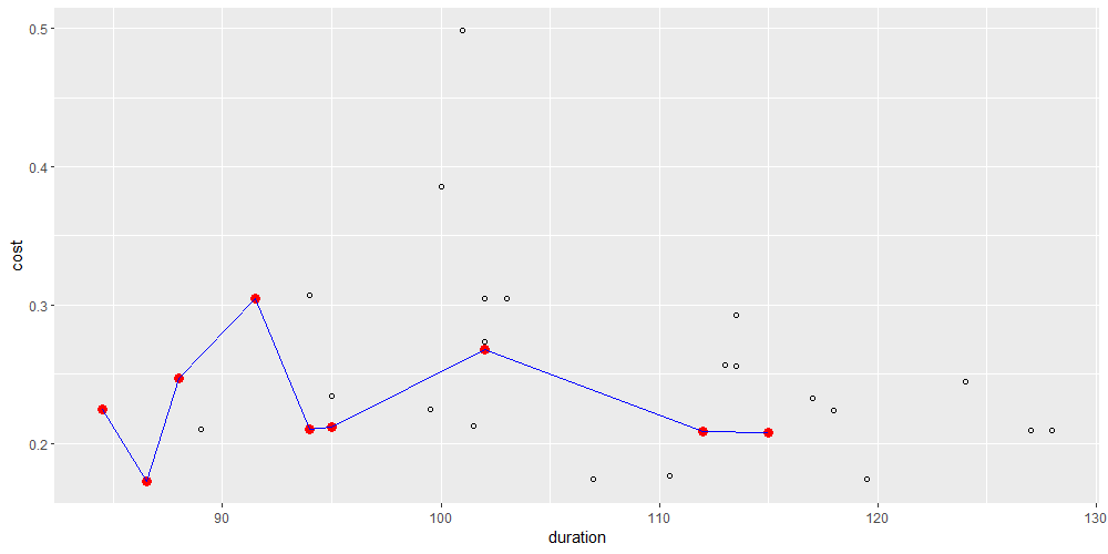
The graph that is shown above we see compares the duration of an intervention to its associated cost. The outcome is logical, as a shorter intervention would have proportionally lower costs due to lower labor and material costs, despite potentially higher single mobilization fees. By contrast, a longer intervention would have proportionally lower mobilization costs but higher labor changes. Therefore, it makes sense that intervention durations lasting sometime between these two extremes would have higher total costs, due to high single mobilization as well as larger total labor and material costs.
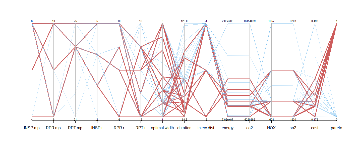
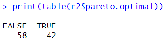
From this second graph, we have 42 optimal solutions (shown in red lines as “TRUE”) with 100 scenarios. These solutions are highlighted as optimal if they were at least as good in all criteria categories and better in at least one category than other solutions (per the pareto.optimal function); we can see that the red lines tend to have higher times between interventions, a higher road width, a shorter intervention duration, and lower values for emissions.
Conclusion
To conclude, with the methods detailed above, we can analyze many different combinations of maintenance, durations and environmental impacts to select the strategies that best adhere to our optimization criteria. In future iterations of the code, we could perhaps also implement another multi-criteria decision making analysis such as the AHP method to narrow down our results, or we could use sensitivity analysis to confirm our final selections. Finally, we would also further regard the impacts of all six systems instead of basing our optimization on the two most critical.