Interpretations
Resulting from the Multi-Objective Optimization, different options vary throughout the different factors, which makes the process of decision making more complicated. In order to get a better overview of the situation, a closer look at the single characteristics of each solution will be provided before generalizing the observations.
1-Energy consumption
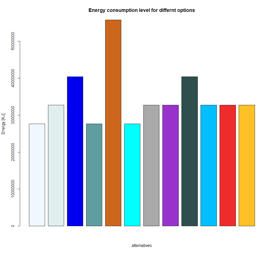
Fig 5.1 : Energy_barplot
Fig.5.1 shows, that options 1, 4 and 6 are the less energy consuming solutions by consuming 27629947.9 kJ while option 5 with a consumption of about 28084155.5 KJ is higher. Option 5 represents the option with the highest amount of energy consumption.
2-CO2, SO2 and NOX emissions
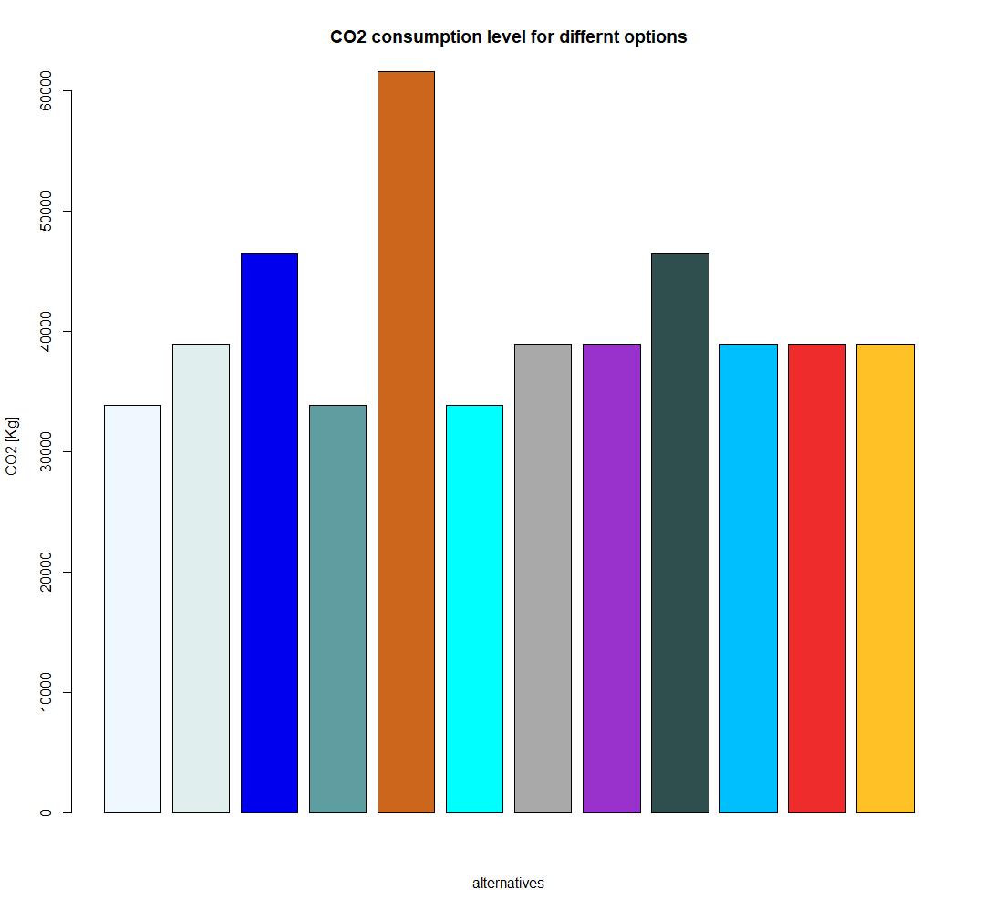

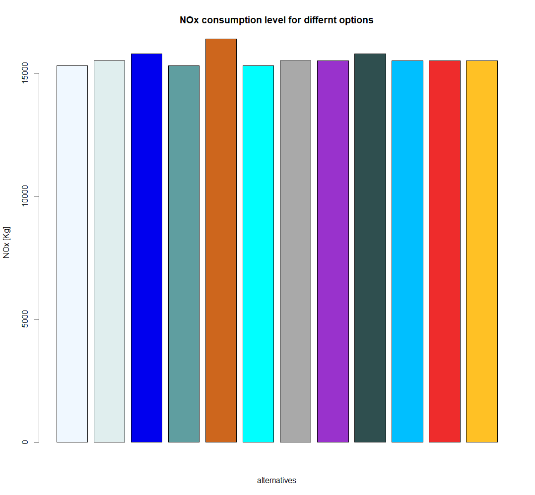
Fig.5.2 displays, that options 1, 4 and 6 with values of 33889.55 kg, 3532.01 kg and 15305.79 kg for CO2, SO2 and NOX are the less greenhouse gases emitting solutions while again option 5 emits the highest values.
3-Time factors
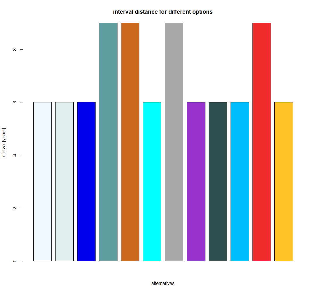
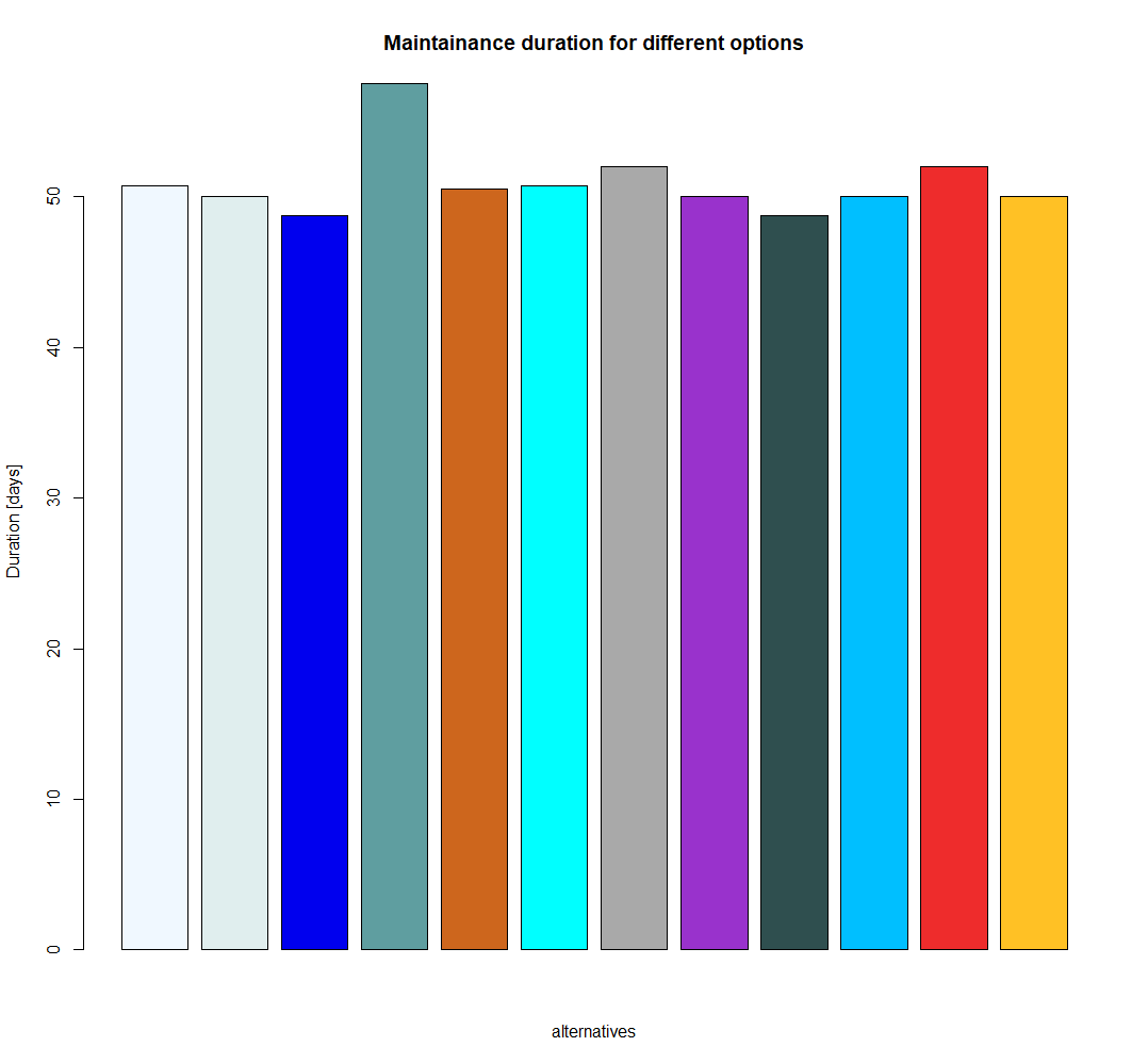
Fig.5.3 reveals that options 3 and 9 involve less maintenance days during the life cycle (48.75 days) while option 4 has the highest number of maintenance days. On the other hand, options 4, 5, 7 and 11 have the greatest time intervals between the maintenance actions with 9 years while the other options amount about 6 years.
4-Economic factors

According to Fig.5.4 Options 1, 4 and 6 turn to be more economical involving 5 360 825 Euros for the whole life cycle, while option 5 is the most expensive with nearly the double costs of 10 019 663 Euros.
All evaluation factors are summarized in the table below:
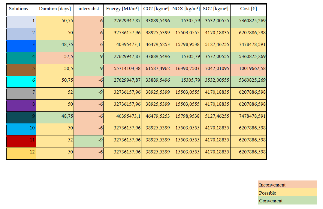
NB: From the table it can be noticed that the following group of solutions are identical.
- 1 and 6
- 2,8,10 and 12
- 3 and 9
- 7 and 11
Although, all options have different input sets of values, the same outputs can still be obtained through different paths. Therefore, the outputs are flexible, meaning that the more the options with the same outputs are, the greater is the flexibility of these outputs. Thus the optimization can be easier run.
Decision Making
The importance of each factor being determined by stakeholders and not designers, induces the distribution of equal weights to the evaluation factors here. So, each factor was rated as a percentage on a scale with reference to the highest value in its column. It resulted to two equations
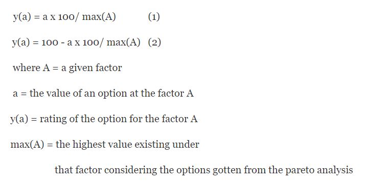
(1) applies to the distance between the interventions, because the higher the value is, the better the maintenance startegy. While (2) applies to factors like the greenhouse gases, the costs, duration and energy. For these the option with the lowest percentage actually reweals the best values for the maintenance strategy.
The graph below shows the ratings of the different options concerning different evaluation factors.
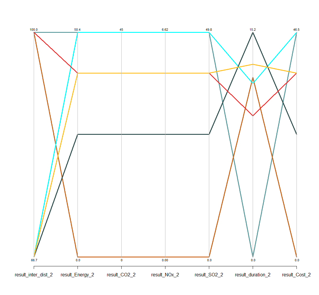
NB:
- Some lines are not visible because the options are identical.
- A Multiple-Criteria Decision Model (MCDM) like AHP and TOPSIS could be conducted in case the stakeholders agree on the weighs of the factors.
Page Navigation
3. Life-Cycle Inventory Analysis
4. Multi-Objective Optimization
5. Interpretations and Decision making