Introduction
This chapter presents an analysis of the multi-objective optimization (MOO) results for the given dataset. Our primary objectives are:
- Minimizing intervention duration to reduce downtime and disruption
- Maximizing intervention distance (efficiency in interventions)
- Assessment of energy consumption and environmental impact (CO2, NOx, SO2)
- Cost-effectiveness
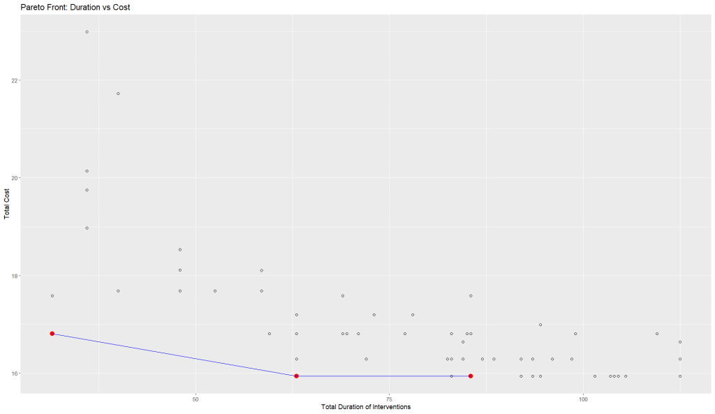
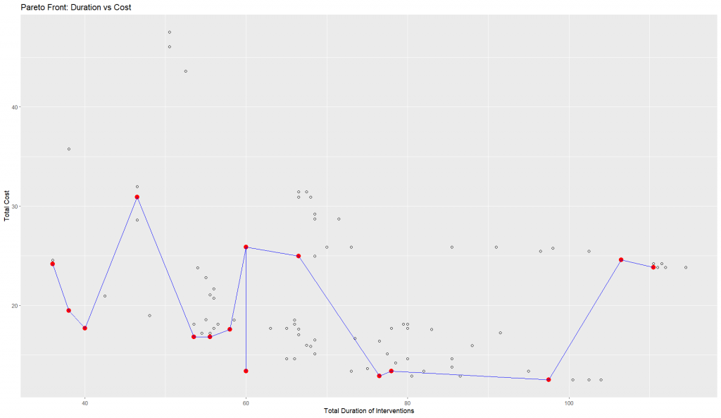
Two different sets of solutions were analyzed: one with fewer solutions (first dataset) and another with more Pareto-optimal solutions (second dataset). A parallel coordinate plot was used to visualize relationships between design parameters and objectives.
Analysis of Best Solutions
We have provided two versions of our multi-objective optimization results:
1. The first version (fewer solutions)
- Contains fewer red lines (Pareto-optimal solutions).
- Easier to interpret because there are fewer overlapping lines.
- May not capture all possible trade-offs well.
2. The second version (more Pareto-optimal solutions)
- Has more Pareto-optimal solutions which mean more trade-offs are considered.
- Denser visualization, making it harder to analyze trends.
- Likely includes more extreme values, offering a wider range of decision choices.
We compared these in terms of quality, interpretability, and effectiveness for decision-making.
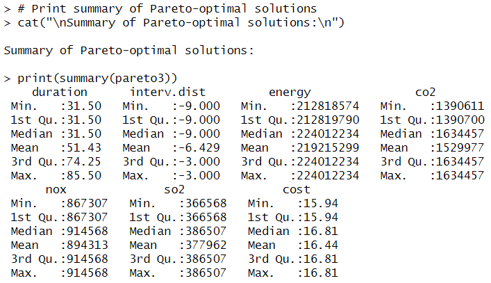
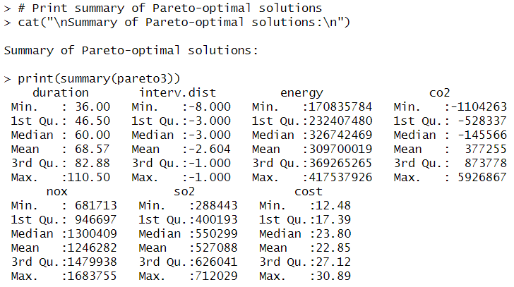
| First Version of Pareto-optimal Solutions(few trade-offs) | Second Version of Pareto-optimal Solution(more trade-offs) |
|---|---|
 |
 |
 |
 |
 |
 |
 |
 |
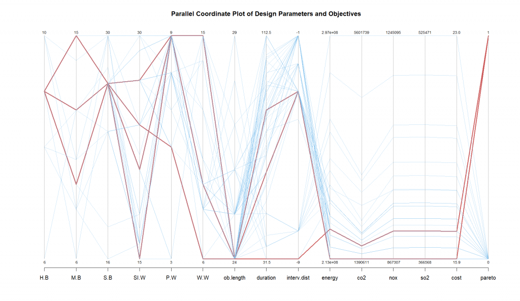
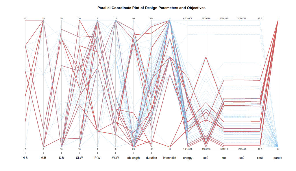
To easily visualize the best solutions, we used a parallel coordinate plot and plotted each parameter along parallel vertical axes. Each line represents a single solution (or set of parameter values), and its path shows how that solution maps to different variables.
The horizontal axis represents different design parameters and objectives, labeled as:
- H.B, M.B, S.B (Building Maintenance Actions)
- SI.W, P.W, W.W (Water Supply Facility Maintenance Actions)
- ob.length (Office Building Length)

- The increase in job opportunities not only leads to a rise in office building floor area and local housing demand but also creates an incentive for incoming students to relocate to the area for education. Based on this interaction pattern, we assume that for every 100% increase in office building capacity, the floor area of student dormitories and residential buildings will increase by 20% and 50%, respectively.
- Student Dormitory: sd.length = 24*(ob.length/24*0.2)
- Residential Building: rb.length = 30*(ob.length/24*0.5)
- Water Supply Facility: wf.length = 40
- duration (Total Intervention Duration)
- interv.dist (Time Between Interventions)
- energy (Energy Consumption)
- co2 (CO2 Emissions)
- nox (NOx Emissions)
- so2 (SO2 Emissions)
- cost (Total Cost of Maintenance and Interventions)
- pareto (Indicates Pareto-optimal solutions: 1 = Pareto-optimal, 0 = non-optimal)
The vertical axis for each variable is scaled independently.
The plot shows trade-offs between objectives using different colors: red lines represent Pareto-optimal solutions that offer the best balance, while blue lines indicate non-optimal solutions. Positively correlated variables show parallel trends, whereas negatively correlated ones intersect. The optimization aims to minimize intervention duration and costs while considering environmental impacts (CO2, NOx, SO2, energy use). The red lines show how different design choices balance these factors. Several variations in certain axes, such as cost and duration, indicate a broad range of feasible solutions, while nearly constant parameters indicate minimal influence on optimization.
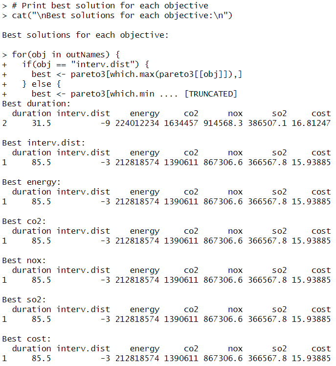
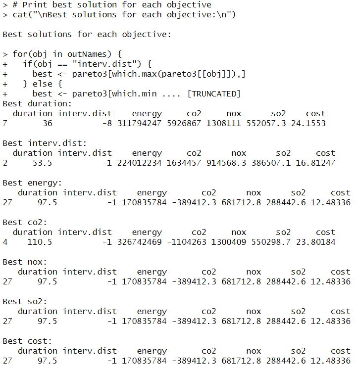
Table 2. Comparison of the Best Solutions for Each Objective
| Objective | Best Duration (First Version) Solution 2 |
Best Duration (Second Version) Solution 7 |
Best CO2 (First Version) Solution 1 |
Best CO2 (Second Version) Solution 4 |
|---|---|---|---|---|
| Duration (years) | 31.5 | 36 | 85.5 | 110.5 |
| Interval dist. (years) | -9 | -8 | -3 | -1 |
| Energy (MJ) | 2.12E+08 | 3.12E+08 | 2.12E+08 | -3.26E+08 |
| CO₂ (kg) | 1,390,611 | 5,926,867 | 1,390,611 | -1,104,263 |
| NOₓ (kg) | 867,306 | 1,308,111 | 867,306 | 1,300,409 |
| SO₂ (kg) | 366,567 | 552,057 | 366,567 | 550,298 |
| Cost (€) | 15.94 | 24.15 | 15.94 | 23.80 |
We examined the difference between the best solutions from both optimization versions we have observed that:
Trade-off Between Duration and Environmental Impact
The newly identified optimal duration is slightly longer (36 years compared to 31.5 years). However, this minor increase leads to higher environmental impact and cost, highlighting a trade-off: reducing maintenance frequency results in greater long-term environmental and financial burdens. Additionally, the updated best CO₂ solution differs significantly (-1.1E+06 vs. 1.39E+06). The second optimization run appears to have identified an extreme trade-off, potentially overemphasizing CO₂ reduction at the expense of practical feasibility.
Exploration of More Extreme Values
Compared to the first run, the second optimization explores more extreme values, offering a broader spectrum of solutions.As we can see the initial run produced a more stable range, the updated results include longer intervention distances, significantly lower CO₂ emissions (-1.1E+06), and reduced costs (12.48B). This expanded solution space suggests a more wide range of trade-offs, suggesting unconventional yet impactful alternatives that assists further evaluation.
Choosing the Best Solution Set
The best solution sets depends on the desired trade-offs and objective. If the decision maker prefers a balanced and stable approach, the first set of solutions will be more suitable. However, if the priority is to achieve more aggressive reductions in both emissions and costs, the second set of solutions offers greater advantages. Given the objective of minimizing duration while maximizing intervention distance, the second solution set that contains more Pareto-optimal solutions is preferable because it provides greater flexibility in selecting the best trade-offs.