Until now we have found two solutions for the duration of the maintenance of the integrated system for the lifetime, and both their values were 14 days, more suitable then initially obtained 104 days.  We were able to receive the Life-Cycle Analysis results for the integrated system, which included the energy used by the various systems, greenhouse gas emissions (CO2, SO2, NOX), as well as repairs up until the end of the system’s lifecycle.

The principal purpose of this multi-objective optimization is to merge separate systems by integrating their maintenance schedules throughout a 120-year lifecycle. The optimization will result in a reduction of expenses while increasing functionality time throughout the integration context.

In more specific terms, the goal is to increase the intervals between treatments while reducing the overall number of interventions and their lengths.

To justify this principal, a FITNESS FUNCTION is introduced and used as an algorithm. The algorithm submits the best set of solutions for the specified objectives Using an initial data set provided by the Fitness Function and a suitability function to form new data sets. Up until the best data set is discovered, these steps are repeatedly iterated.

A predetermined range of intervention periods for each component as part of the maintenance planning defines the input parameters for the fitness function.

• Interventions durations for the building:
  • 10 ≤ CRF≤ 20
  • 2≤ M ≤ 8
  • 24 ≤ CR ≤ 36
• Interventions durations for the bridge:
  • 2 ≤ SDO≤ 6
  • 2≤ M ≤ 8
  • 24 ≤ DR ≤ 36
  • 5 ≤ SR ≤ 10
• Interventions durations for the Roof:
  • 5 ≤ CF≤ 15
  • 15 ≤ RT ≤ 25
  • 50 ≤ RR ≤ 70
• Interventions durations for the Road:
  • 5 ≤ PO≤ 15
  • 2≤ M ≤ 10
  • 15 ≤ PR ≤ 2

Additionally, the integrated system’s width integration parameter will be based on a value produced by a genetic algorithm, therefore it will likewise vary within a range and iterated. The parameters of the overall duration, the shortest distance between two successive interventions, the energy consumption, and the quantity of emissions such as CO2, NOx, and SO2 as well as their associated cost will be determined as the output of the fitness functions. The Pareto Frontier is then used as the best solution to plot the resulting data set.

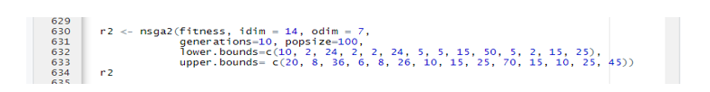
Every time the R-Code is run, a fresh set of results is produced since the Genetic Algorithm’s random nature causes its input parameters to be set randomly. But the optimal answer is discovered for every set of input parameters. An initial data set with 14 different input parameters (idim) is processed over the course of 10 iterations (generation) to produce a new data set with 7 output parameters (odim) out of 100 options (popsize). Refer the following image.

 

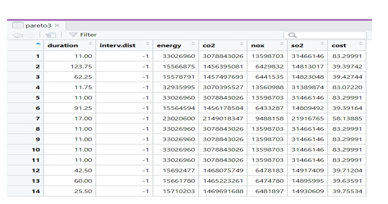
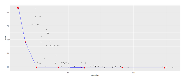
Now, in order to enhance the maintenance plan the maintenance period and/or lifecycle expenses should be minimized. To achieve this aim, a pareto front is being expressed graphically to analyse different alternatives. There are a total of 14 options produced, which are displayed in the diagram below.

 

 

However, they are not the only objectives, additional elements (such as emissions, energy use, and interventions) need be taken into account for each of the 14 alternatives. In the figure below, the values of every element that made up the choice are displayed.

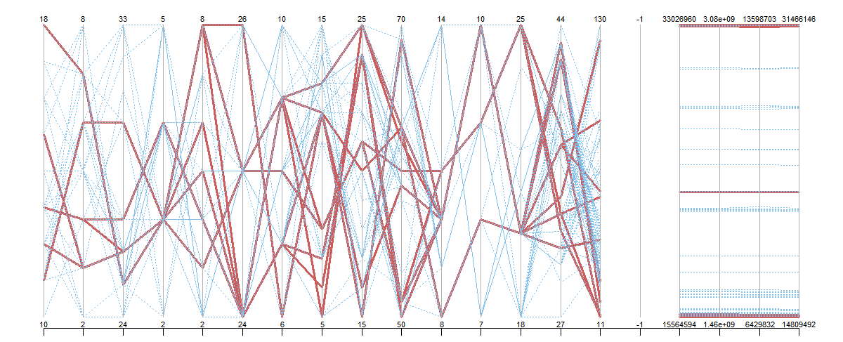
Every Alternatives are displayed by Blue and Red Colored Lines and each optimized option is visualized with a color Red. The fact that certain solutions utilize more energy or emit more greenhouse gases than others is obvious. Depending on the scope and aim that have been established, these considerations may influence the decision of stakeholders.

Following are the results of the Best Suitable alternatives that we achieved from the above Optimization and can be used for the decision making of the stakeholders.