Maintenance Strategy for individual systems
Maintenance actions are critical in ensuring the proper functioning and longevity of civil systems, such as buildings, roads, bridges, water supply systems, and other infrastructure. There are several reasons why maintenance is important:
- Safety: Regular maintenance helps to identify and fix potential safety hazards, such as structural weaknesses, leakages, and other issues that can pose a threat to people and the environment.
- Longevity: By regularly inspecting and repairing civil systems, maintenance actions can extend their lifespan and prevent costly replacements or overhauls in the future.
- Cost-effectiveness: Regular maintenance is often less expensive than having to repair or replace a system after it has broken down or failed. By keeping systems in good condition, maintenance actions can help to avoid expensive repairs or replacements in the future.
- Reliability: Maintenance helps to ensure that civil systems are reliable and function as intended, reducing the likelihood of disruptions or failures. This is particularly important for critical systems such as water supply or transportation networks.
- Compliance: Maintenance is regularly required to ensure compliance with regulations and standards, such as building codes or environmental regulations. By performing regular maintenance, organizations can ensure that their systems are in compliance and avoid costly penalties or legal action.
If we look at our energy supply system in a remote area, it becomes especially clear how essential maintenance actions are, since the basic need for warmth depends on the functioning of the system. To guarantee this needed reliability, the following regular interventions will need to be put into practice. If you want to know more about the different interventions, look into the descriptions of the subsystems on this website.
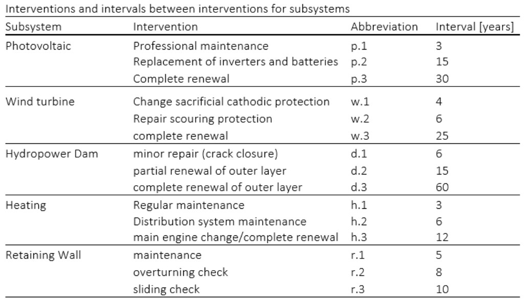
As already pointed out previously, our system consists of five different subsystems, which all have different lifetimes. The following table illustrates these.
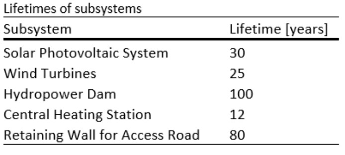
To take this into account while planning the maintenance of the whole system, we calculated a total lifetime of 100 years, given by the lifetime of the Hydropower dam. We assumed that the Solar Photovoltaic System, the Wind Turbines, and the Central Heating Station require a complete renewal after their shorter lifetime is over. We implemented this by treating the complete renewal as an intervention on its own. The following timelines visualize the specific maintenance program for the individual subsystems.
Integrated maintenance planning:
Optimizing maintenance planning for a system with multiple subsystems is especially important because it helps to coordinate and synchronize maintenance activities across all subsystems. This can help to minimize the impact of maintenance activities on the overall system and reduce the likelihood of failures or unplanned downtime.
In this part of the analysis, we want to concentrate on how we can bundle maintenance actions of the subsystem to have in total fewer days of interventions during the lifetime of the system. To do so, we assumed that each intervention for each subsystem has a range of years in which it can take place and a duration of the day each action needs. These numbers are displayed in the following in Figure 4.
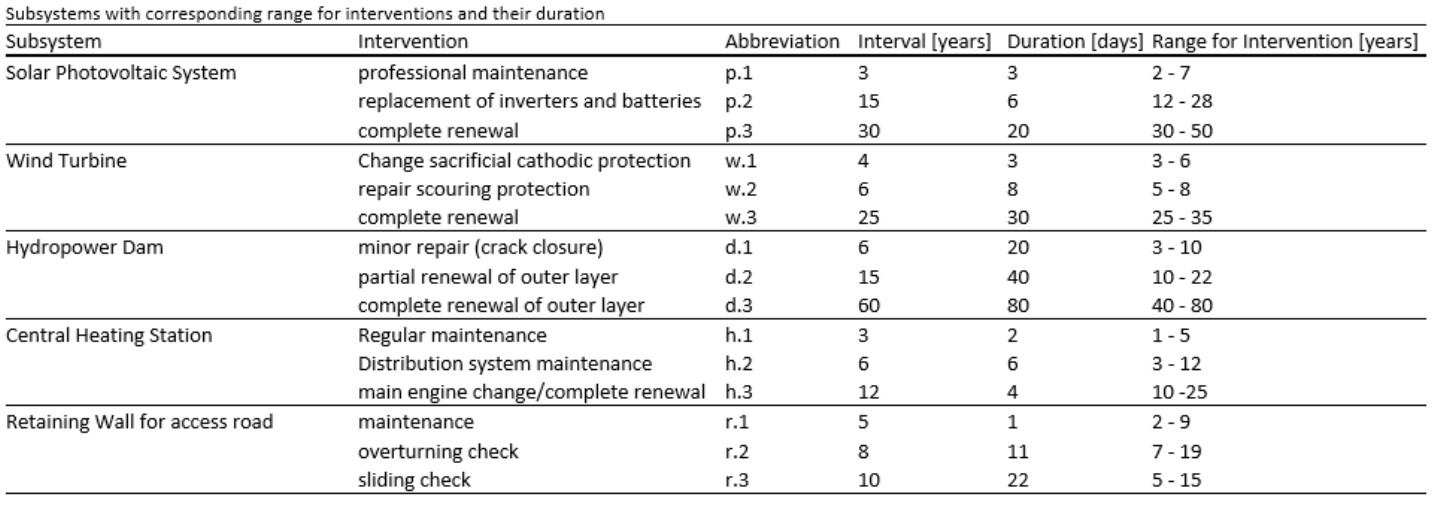
To make an example, this table shows, that the professional maintenance of the Solar Photovoltaic System can take place two to seven years after the last professional maintenance and this intervention takes 3 days.
When considering the overall maintenance procedure of a meta-system, the semantic relations between the individual system functions make the bundling of maintenance functions an important task for the planning engineers and system managers. This can be seen by comparing the number of maintenance days for 100 years of the individual maintenance strands of the subsystems (Figure 5) with that of the overall system for the same lifetime (Figure 6).
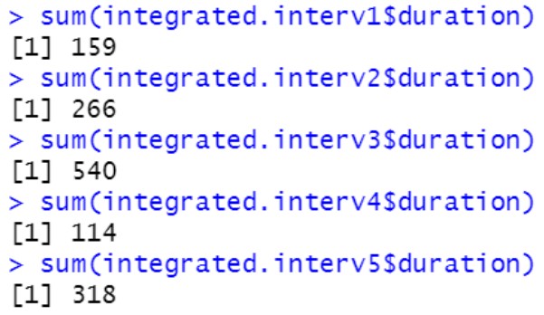
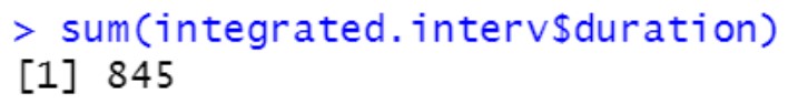
The sum of the individual maintenance plans for the subsystems is 1397 days. Compared to the bundled maintenance plans for the overall system of 845 days, we saved 552 days, which is 1,5 years. This is a strong improvement. The work on the system which needs to get done is the same, but there are now more days in which we don’t have any interventions on the system, which means during the days of the interventions resources are used more efficiently, which means costs can be saved.
We achieve this with the help of the lifetime function of our R-script. Maintenance tasks initiated in the same cycle, are bundled.
In our system, the maintenance requirements for different subsystems vary greatly, as evidenced by the difference in maintenance actions for the Hydropower Dam and the Photovoltaic. As a result, there may be a need for optimization in the specification of individual maintenance measures. To effectively bundle and combine these measures, similar prerequisites should be established. Therefore, little synergy can be exploited from this bundling for the execution of individual measures due to the diversity and also physical separation. Nevertheless, the total repair time for the entire system is a good indicator for evaluating the entire system in terms of the expected duration of the repair work. These characteristic values can be used, for example, in earlier design phases to make statements about the resources to be roughly planned for the life cycle for any system downtimes and the required maintenance periods.
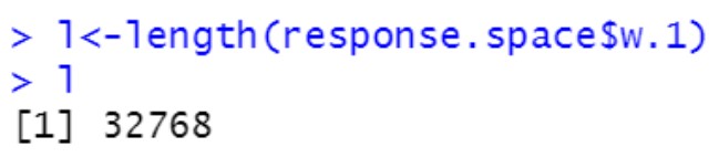
These initial figures can be further optimized by modifying the “duration” and “distance between intervention” parameters of the data examined for the individual systems. Limitations (low(), high()) are set for these parameters, which lead to a higher efficiency of the total system usage by applying these functions to our combined timelines. The quality of our data and also results are measured at this point by the n.grid variable, which leads to the extent of the created timeline combinations, which are included in this consideration. Due to the system integration of 5 subsystems and our available computing resources, we have set this parameter to 2 in order to generate results at all. For this, we got 32.768 different combined lifetime scenarios.
The graphical distribution of solutions in our case has been analysed and based on this analysis, the probability of finding a better solution using this method appears to be low when compared to the computational power. It should be noted that the computational power in this context corresponds to the number of solutions currently generated. In reality, however, it would probably be worth the effort to invest in more computing power, since the savings of a few measures and maintenance days alone would cover the cost of additional computing power. By performing several runs with n.grid = 2, it was found that the deviation for the Pareto solutions was about ± 12 for the duration and ±5 for the dist.inter. This deviation can be used to roughly assess the accuracy of one’s own data analysis. As evidenced by the differences in the magnitude of the results, the expected gain (low(dur)) is likely, not substantial when increasing the value of n.grid compared to the original values for the duration of our static timelines.
It is expected that the gain (low(dur)) will not be significant when increasing the value of n.grid, as indicated by the comparative magnitude of results in Figures 8 and 9.
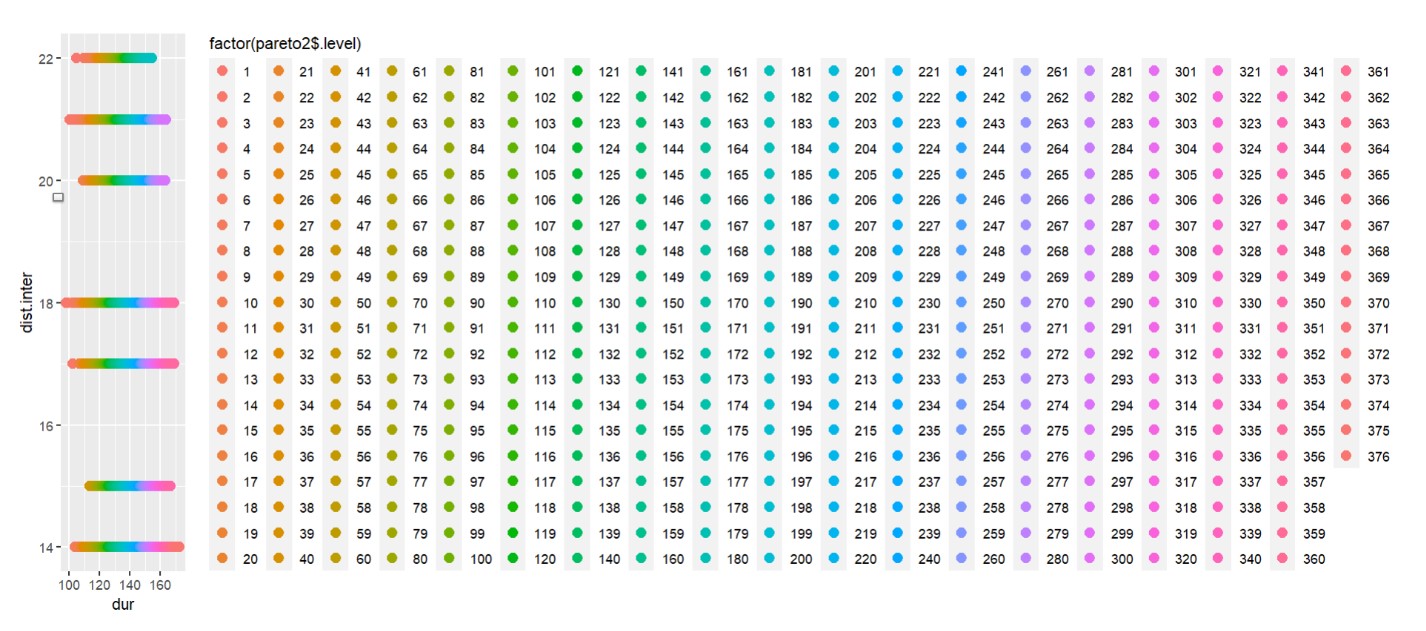
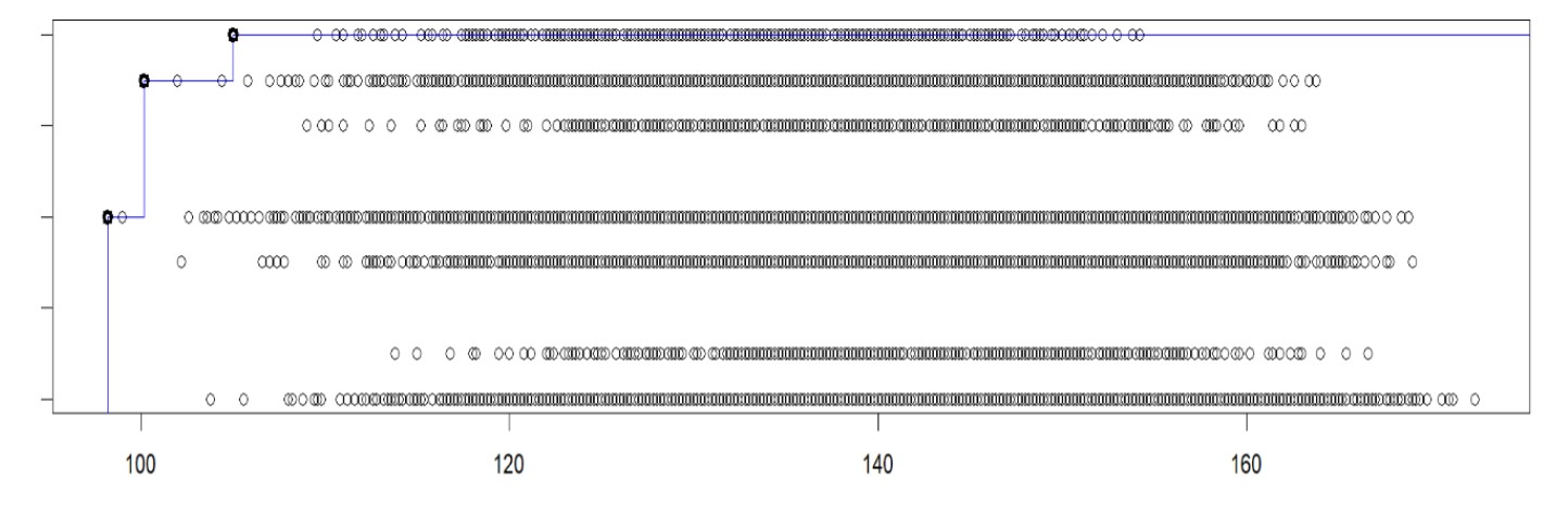
The graphical results represent the distribution of the different scenarios with respect to variables duration and dist.inter. What we want to achieve is the lowest duration of overall intervention days and the highest possible amount of years between the interventions. In Figure 10 the Pareto solutions can be taken from this result set. These represent the solutions for which the improvement of one variable would worsen the other. They are also called the Pareto front.
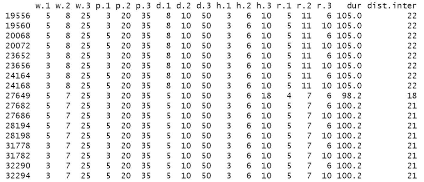
As displayed in Figure 8 there are 17 different solutions on how to plan the maintenance actions in their given possible range. These 17 different solutions lead to three different combinations of duration and distances between interventions. We either have 105 days and 22 years, 98 days and 18 years or 100.2 days and 21 years of duration of interventions and distances between them. The following plots visualize the duration and distances of the different combinations of interventions (Figure 9) and the Pareto front, which shows our results (Figure 10).
Thus, a compromise solution can be found that takes both variables into account. Accordingly, depending on the value of the two variables considered in relation to each other, fine adjustments can still be made in the decision-making process for the optimal solution of the implemented task. Using this method, one can gradually approach multi-objective problems by first applying the Pareto function to find the best possible compromise solution. It can then be determined which of the solutions with which the optimal value of one of the variables is ultimately more important, and the decision can then be made on this basis. However, this only works well for two to three variables. A multi-criteria decision matrix would then be necessary in order to make a targeted selection from several Pareto solutions.
The minimization of this duration quantity provides on the one hand a maximization of the system’s reliability and usability since the operating time is increased in comparison proportionally to the use/lifetime. On the other hand, the simultaneously occurring temporal synchronization of measures leads to a synergy potential. The maximization of maintenance interval times for the entire system ensures that the bundling of measures is primarily designed for larger maintenance measures and not many smaller measures characterizing the maintenance plan.