Objectives

To ensure long-term structural integrity and operational efficiency, our objective is to maximize the time between minor and major interventions while minimizing downtime through optimized scheduling. Besides, it reduces disruptions while enhancing resource efficiency by aligning HVAC, MEP, fire inspection and structural maintenance. For instance, scheduling HVAC filter replacements together with the inspection of fire safety elements limits the shutdowns that must be repeatedly performed. The engineering analysis of material degradation rates, their failure probability, and system interdependencies enables preventive interventions at an optimal intervention interval, enabling the maintaining of building performance, reduction in operational costs, maximization of occupant safety, and maintaining conformance to standards, thus extending the life span of infrastructure.

First Maintenance Strategy

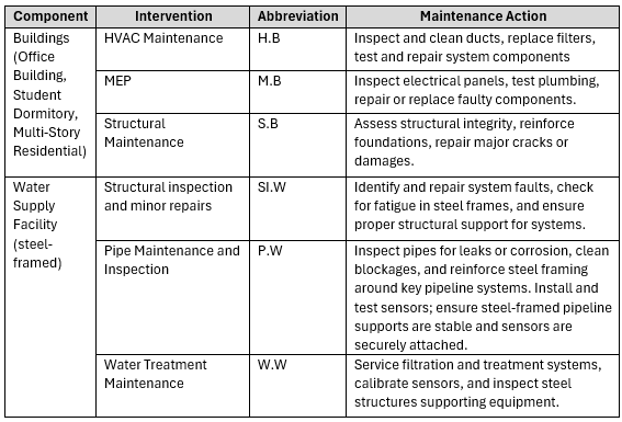
The diagram in Figure 1 presents an interconnected system of three buildings—Residential Building, Student Dormitory, and Office Building—linked to a central Water Supply Facility. Each building serves specific purposes: housing for locals, affordable living for students, and workspace for economic activity. Shared systems like MEP (Mechanical, Electrical, and Plumbing), HVAC, and water supply support safety, comfort, and functionality across all buildings. The water supply ensures clean water for daily use and fire safety systems, making it critical to overall operations. 

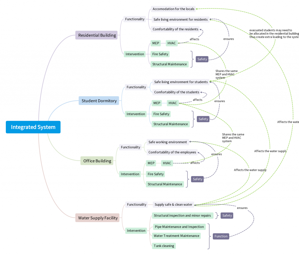
Figure 1: Intervention-Functionality Relationship in Integrated Maintenance

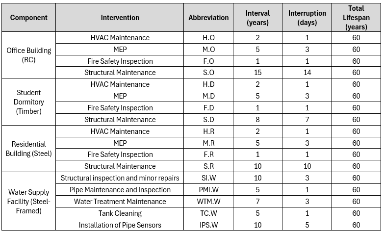
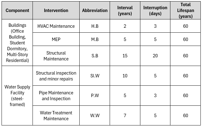
According to Deetman et al. (2020), the overall global estimated lifespan for residential and service-sector buildings is 60 years. Therefore, we set the total lifespan for each building at 60 years, with a strong emphasis on preventive maintenance to enhance durability, reduce failures, and optimize long-term performance.

Table 1: Maintenance Schedule for First Strategy

 

Maintenance Timeline from the start of usage until the end were presented below:

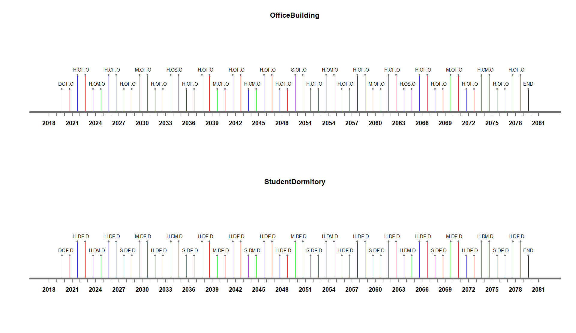
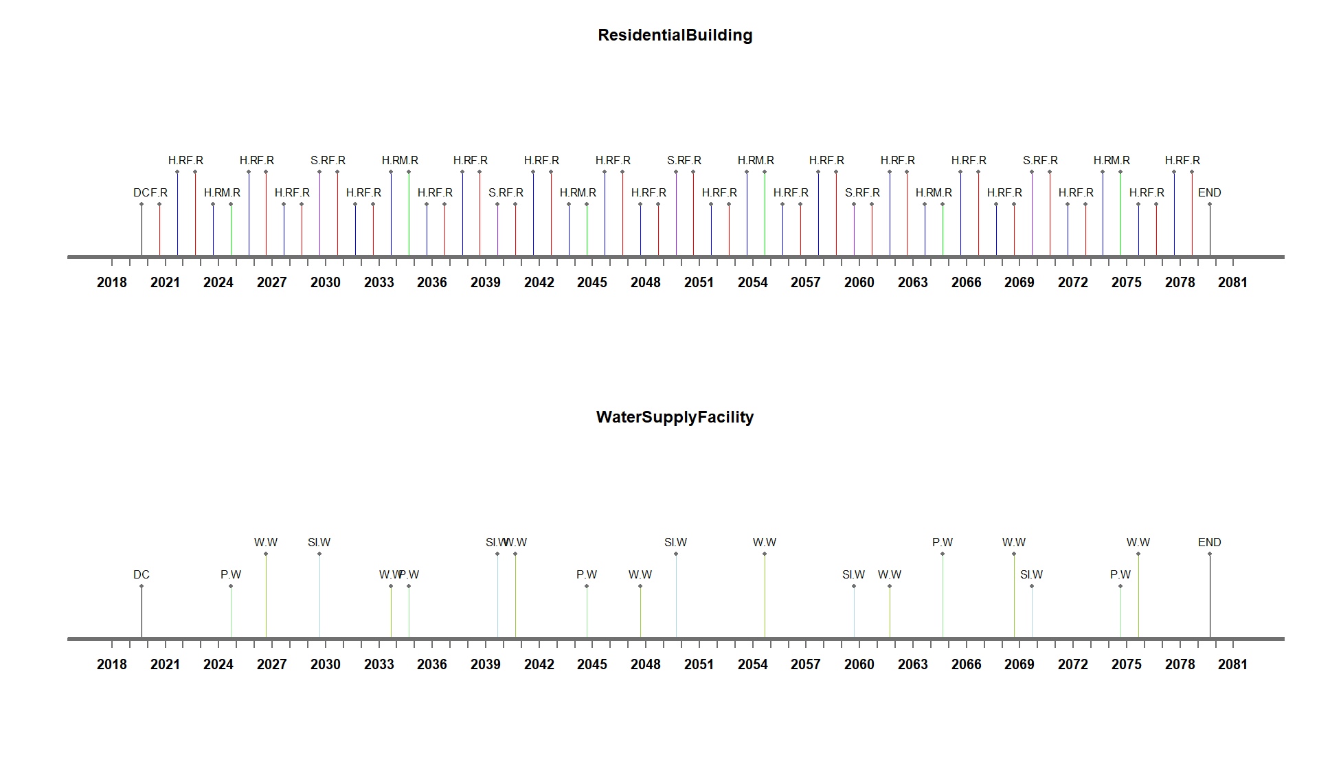
Figure 2: Intervention timeline of individual systems under 1st maintenance strategy

Figure 3: Total duration of the interventions under 1st maintenance strategy

The first maintenance strategy yielded 17 interventions and 317 days of total durations as similar interventions are very close to each other. Therefore, the computational time had been more than five hours. Hence, there comes the need of optimizing the first strategy to reduce the complexity and overall downtime.

Interdependencies and Engineering Reflections

• Shared systems create efficiency but also increase dependency. Maintenance or disruptions in one building, such as HVAC or plumbing repairs, can affect others. For example, replacing HVAC ducts in the dormitory could disrupt air quality in the office and residential buildings. Water supply interruptions due to pipe repairs or tank cleaning may impact fire safety and sanitation across all buildings, creating operational delays and discomfort.
• Structural repairs, like scaffolding for the residential building, could block access roads and disturb the dormitory or office building. Coordinated maintenance is crucial to reduce such disruptions. Adding redundancies, like localized water storage or independent fire systems, can enhance resilience. Sensors for water leaks or HVAC performance monitoring can ensure predictive maintenance, minimizing failures. Lifecycle assessments of materials and systems across all buildings can lower costs and improve durability and reliability in the integrated system.

Second Maintenance Strategy (Optimization of the First Strategy)

To optimize the maintenance plan for less overall downtime, we adjust the intervention intervals to coincide with others for a more efficient second maintenance strategy. Such examples include the inclusion of Fire Safety Inspection in HVAC Maintenance since it is very common for companies in the industry to handle the two together. Similarly, since Tank Cleaning and Pipe Sensors form part of the piping system and their maintenance cycles are similar, ranging from 5–7 years, they have been grouped under Pipe Maintenance to avoid separate interventions with a view to ensuring system reliability.

Table 2: Maintenance Actions for Building and Water Supply Systems 

As shown in Figure 4, the optimized maintenance strategy integrates the three buildings into one plan that combines HVAC, MEP, and structural maintenance. Instead of having separate inspections, a single check for fire safety and HVAC across the buildings cuts downtime, keeps systems running with smooth operation, and ensures durability in the long run.

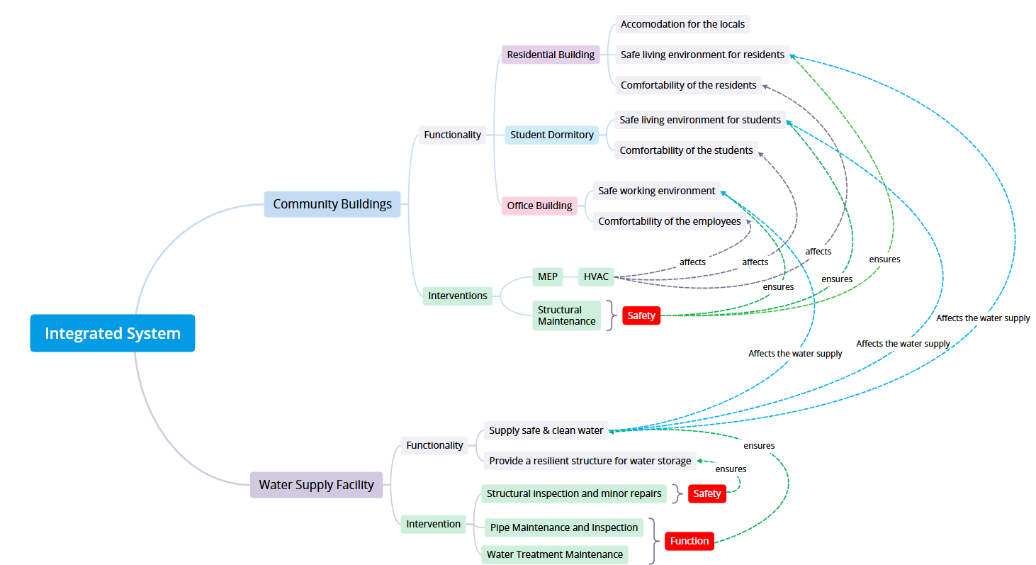
Figure 4: Intervention-Functionality Relationship in Optimized Integrated Maintenance

Then we define the maintenance schedules (frequency and durations) for combined interventions of all three buildings and separately for the water supply system.

Table 3: Second Maintenance Schedules for Buildings and Water Supply Systems

The maintenance frequencies and durations for building systems and water supply facilities are established based on members’ engineering experience, aligning with industry standards and research to ensure optimal performance and longevity. For instance, regular HVAC maintenance is essential for efficient operation and to prevent system failures. Similarly, annual fire safety inspections are standard practice to ensure compliance with safety regulations and the proper functioning of fire prevention systems. In water supply facilities, regular cleaning of water storage tanks is recommended to prevent contamination and maintain water quality. The U.S. Environmental Protection Agency suggests that most utilities employ a cleaning interval of 2 to 5 years. As shown in Figure 5, by applying this optimization, the total maintenance duration is significantly reduced by nearly 40%, decreasing from 315 to 195 days. This improvement greatly enhances the efficiency of maintenance planning.

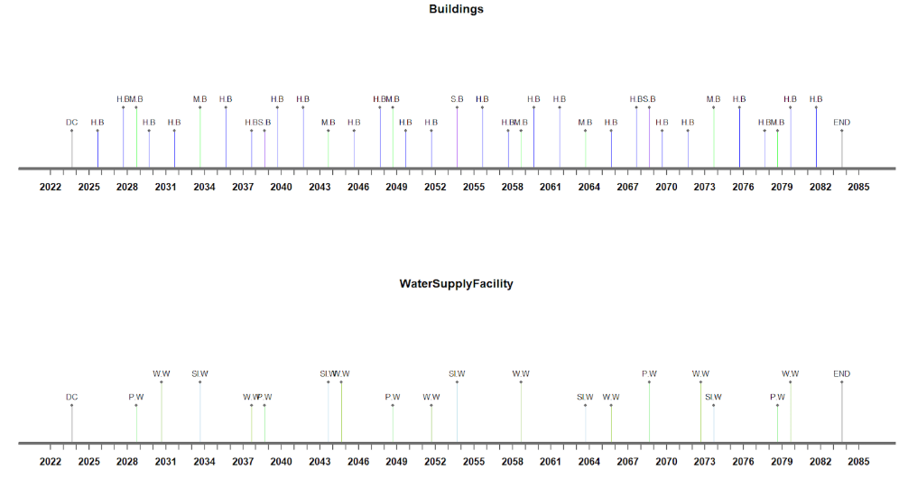
Figure 5: Intervention timeline of individual systems under second maintenance strategy

Figure 6: total duration of the interventions under 2nd maintenance strategy

 Third Maintenance Strategy

For the third strategy, we change the intervals of the maintenance actions to test how different frequencies affect the system performance and cost. According to the industrial maintenance practices, companies often adjust maintenance schedules based on the factors like equipment wear rates, cost efficiency, labor availability and failure risk assessments. For example, MEP requires frequent checks, while structural components like beams and columns can last longer before major repairs. Adjusting intervals lets us compare different strategies to find the most practical, cost effective and optimized maintenance approach.

Table 4: Third Maintenance Schedules for Building and Water Supply Systems

 

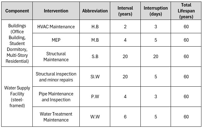
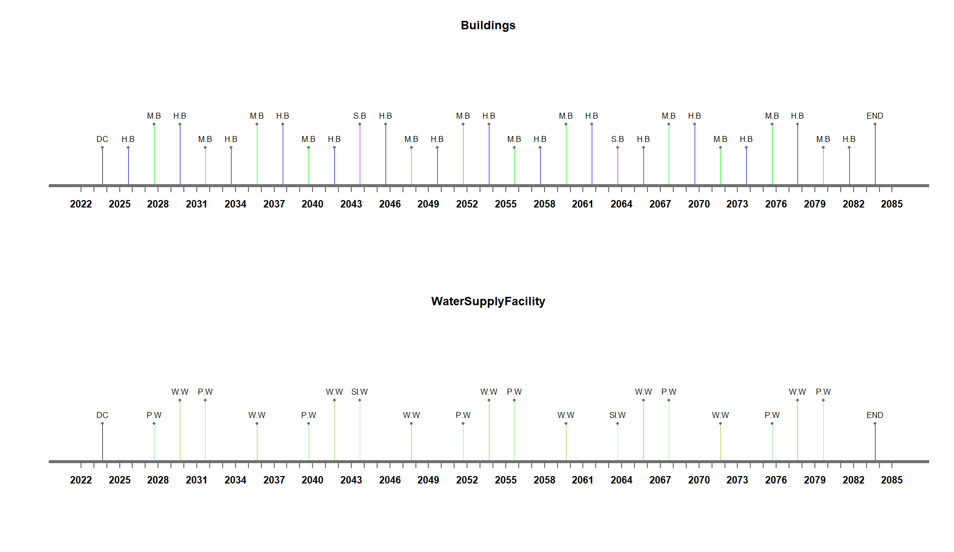Figure 7: Intervention timeline of individual systems under 3rd maintenance strategy

Figure 8: Total duration of the interventions under 3rd maintenance strategy

As observed from Figure 7, the total downtime duration was significantly reduced from 195 to 155 days, achieving a reduction of over 20%. This is because instead of overlapping multiple interventions with the same period, we spread them out to prevent too much downtime at once. These changes obtained a better resource allocation that reduces the  labor congestion and minimizes the impact on the building operations.

Design Space Exploration

To explore more maintenance strategies, a design exploration—using an n.grid value of 5 to regulate the size of the design space being explored—was performed. Here are the ranges of Intervention Events for exploring more scenarios by automating the process:

• Building
  • 2 >= H.B <= 10
  • 5 >= M.B <= 15
  • 15 >= S.B <= 30

• Water Supply Facility (Steel-Framed)
  • 15 >= SI.W <= 30
  • 1 >= P.W <= 10
  • 5 >= W.W <= 15

The frequency ranges are based on engineering judgments. For example, HVAC (2–10 years) is chosen because filters and mechanical parts degrade quickly, due to which they require frequent maintenance. Well-maintained systems can extend up to 10 years. On the other hand, Structural Maintenance (15–30 years) relates to slower deterioration because reinforced concrete and steel require fewer interventions but still need periodic inspections to prevent major failures.

The outcome is shown in Figure 9 and it has resulted into a total of 176 maintenance strategies, while each point represents a unique strategy. As shown in the pareto plot, these can be categorized into three different groups based on the differences in distance between interventions and their total duration (from bottom to top):

• Short Interval, Long Total Duration (dist inter ≈1.0, dur 60–160): Very frequent interventions with the shortest spacing and very high frequency of maintenance. The total duration of maintenance can be highly variable. Such a maintenance strategy can be followed in independent sub-systems, where the maintenance activities are performed separately.
• Moderate Interval-Medium Total Duration (dist inter ≈2.0, dur 100–120): A balanced trade-off where the spacing between interventions is moderate. The total duration of maintenance is mostly between 100 and 120, thus providing a very stable operational schedule with intervention frequency manageable.
• Long Interval-Short Total Duration (dist inter ≈3.0, dur <100): Least frequent interventions while the total duration of maintenance remains below 100, suggesting quick but infrequent interventions that minimize losses. This is suitable for systems where each subsystem is tightly interconnected.

However, the optimal solution is quite difficult to visualize as they show almost the same shade of color. Therefore, we will use another visualization option to identify the best solution depending on our set preferences.

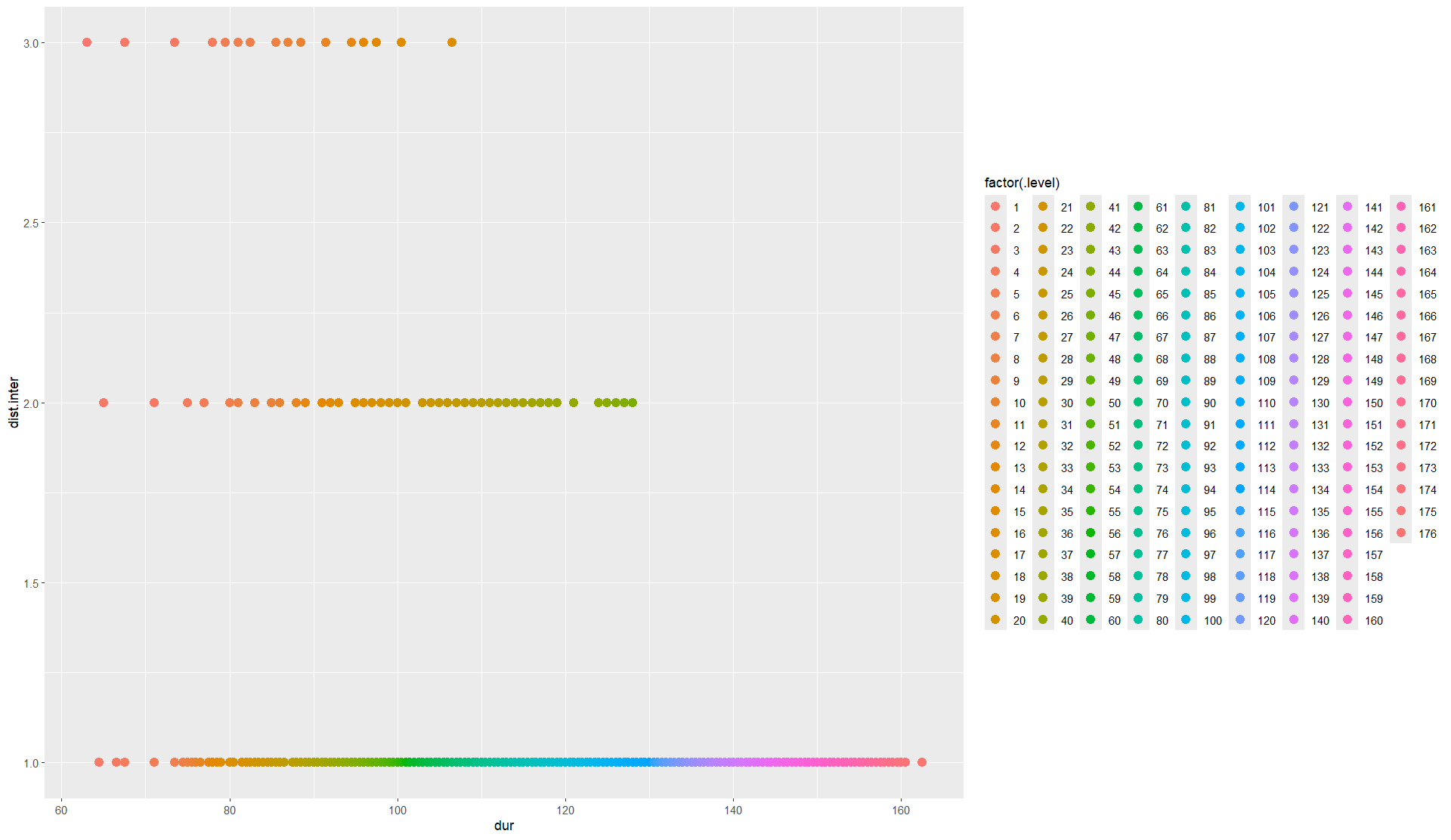
Figure 9: Pareto frontier

Figure 10 shows the Pareto frontier and we can easily visualize which is the best solution. The blue line represents the Pareto frontier, where the dark black point in the top-left corner represents the best alternative based on the lowest duration and highest interval. On the other hand, the figure with the black point at the bottom-right corner gives the solution with the highest duration and the lowest distance of interval. This result will be further used for the Multi-Objective Optimization.

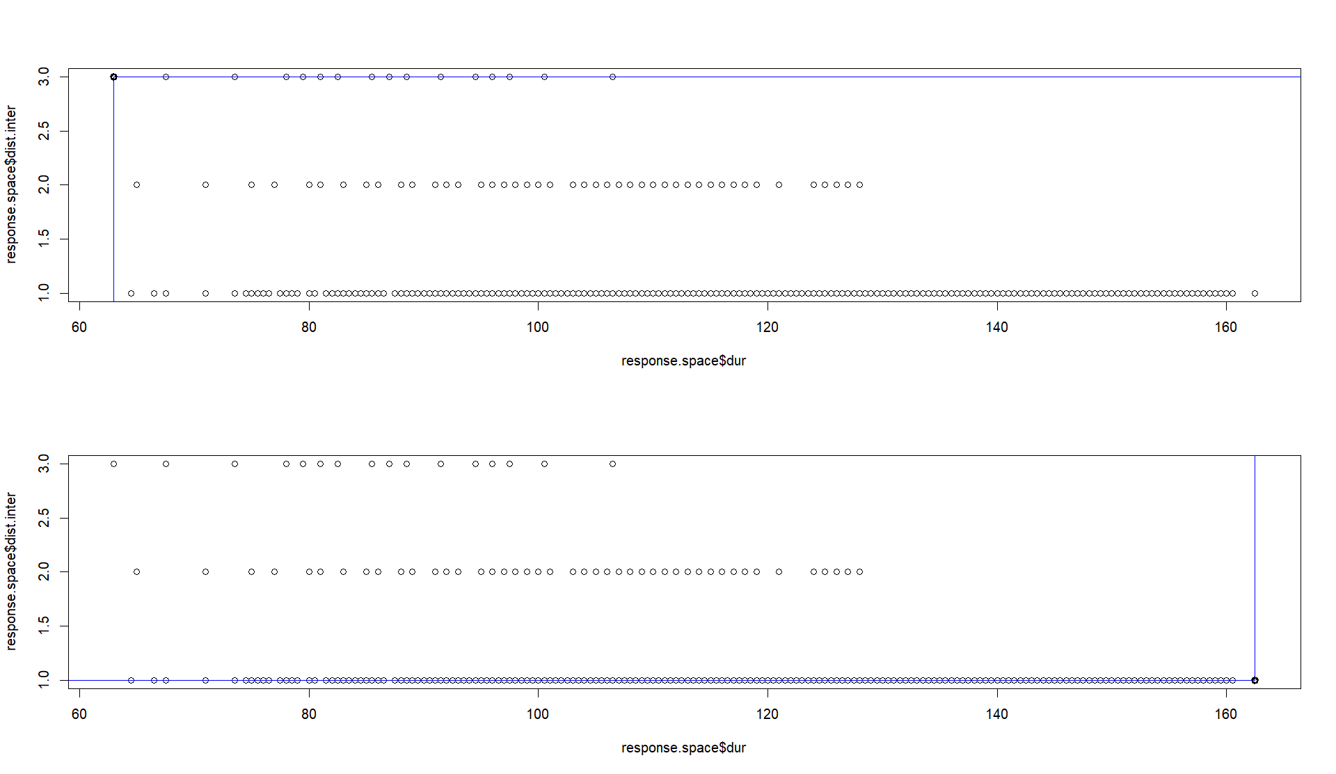
Figure 10: Pareto frontier with different preferences

---

| Main Page | Introduction | Integration Context of the Civil Systems | Integrated Maintenance Strategies | Life Cycle Analysis | Multi-Objective Optimization | Engineering Reflections and Recommendation |