Multi-Objective Optimization (MOO) relies on the optimization of functions which may have conflicting parameters. As such, there is no single optimal solution, but instead multiple best solutions which constitute the Pareto front. These solutions have the characteristic that one of the objectives cannot be improved without worsening another objective (Yao et al, 2023). These solutions are considered non-dominated by each other.
The R code uses NSGA-II, a genetic algorithm for the multi criteria optimization of the following six objectives:
- Total intervention duration
- Minimum intervention distance
- Energy consumption
- CO₂ emissions
- Water usage
- Total cost
In the following table, the examples of the Pareto optimal solutions are shown quantitatively. The bold values show the best values of the listed solutions. As can be seen, it is possible to optimize two objectives (for example, energy and cost), but in this case not more than two. The solution which has the lowest duration of time in maintenance, 40.5 days has the best service score, at only 0.0028% of the lifetime spent offline. However, it scores relatively worse in resource consumption and cost categories. This outcome can be related back to the end users of our project, maintenance planning strategists who must weigh the data and prioritize either service level or resource consumption/cost objectives, given that there is not one solution that prioritizes them all.
Table 1: Solutions to the code which optimize the input objectives
| Duration (days) | interv.dist | energy | CO₂ | H₂O | Cost (billion EUR) |
| 56.5 | -1 | 969573467 | 6133.831 | 890.7919 | 0.1242664 |
| 47 | -1 | 969573467 | 6387.66 | 1038.0754 | 0.1242732 |
| 55 | -1 | 353878147 | 7149.147 | 1479.9257 | 0.0454848 |
| 49.5 | -1 | 1585268786 | 5626.173 | 596.225 | 0.2030617 |
| 47 | -1 | 969573467 | 6387.66 | 1038.0754 | 0.1242732 |
| 40.5 | -1 | 1791020251 | 5144700.71 | 4853759.613 | 0.3712642 |
| 45 | -2 | 1790963897 | 4293052.974 | 4045053.423 | 0.3477393 |
| 45 | -2 | 970093158 | 5143939.223 | 4853317.763 | 0.266165 |
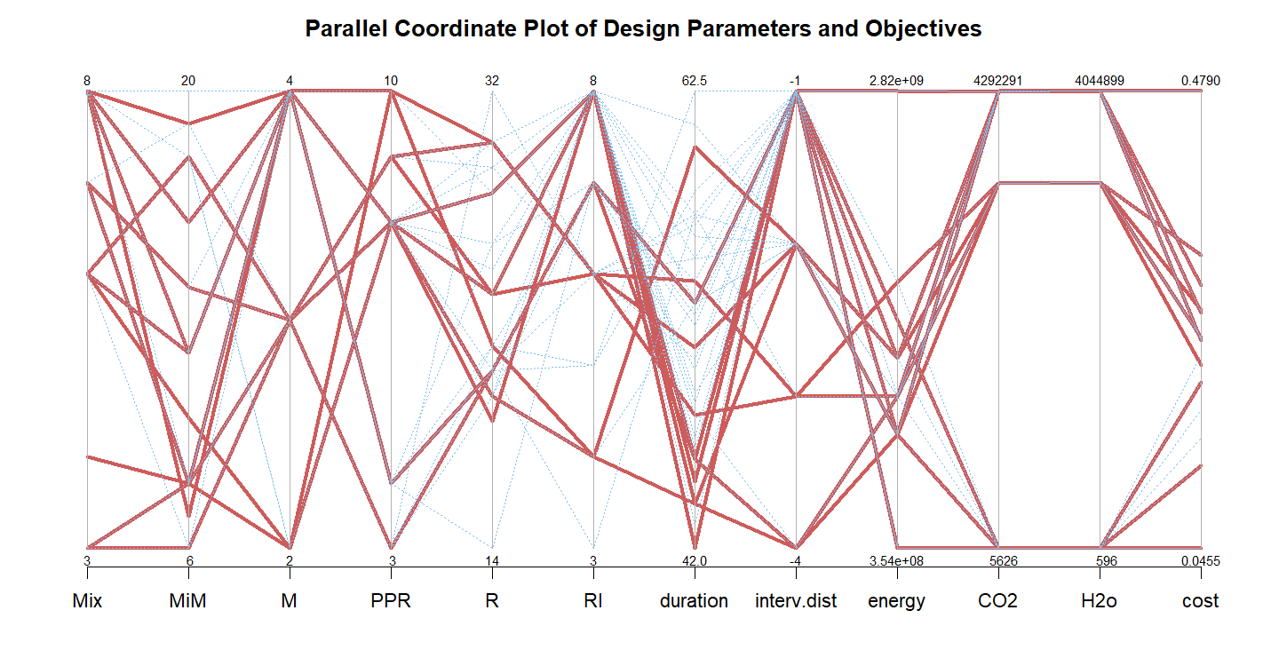
One of the strengths of MOO is in analyzing life cycle objectives which in effect are the sum of many more specific objectives (De Weck, 2004). In the case of this project, those are most prominently reliability and maintainability. We are illustrating the relationship between short term objectives such as cost, resources use and downtime and these more abstract life cycle objectives, with the decision making still relying on the end-user in order to determine which of these objectives should be prioritized. Figure 1 below shows a graphical summary of all the Pareto-optimal solutions, where the straight lines connecting the CO₂ and H₂O categories show how these solutions are often linked in being optimal or equally sub-optimal.
Figure 1: Parallel coordinate plot of Pareto optimal solutions (red) to visualize the trade-offs necessary to optimize
Sources:
De Weck, O. L. (2004). Multiobjective Optimization: History and Promise [Invited Keynote Paper, GL2-2]. Third China-Japan-Korea Joint Symposium on Optimization of Structural and Mechanical Systems, Kanazawa.
Yao, H., Xu, Z., Hou, Y., Dong, Q., Liu, P., Ye, Z., Pei, X., Oeser, M., Wang, L., & Wang, D. (2023). Advanced industrial informatics towards smart, safe and sustainable roads: A state of the art. Journal of Traffic and Transportation Engineering (English Edition), 10(2), 143-158. https://doi.org/10.1016/j.jtte.2023.02.001
← Previous Page: Life Cycle Analysis
