As the perspective broadens and more systems are designed together in a coherent integration context, the scope of different important possible objectives widens as well. The famous triangle of objectives: cost, time and quality can be complemented with objectives concerning the emissions of greenhouse gases. Many more objectives could be pertinent, but for the local transport system six objectives were chosen. The two concerning the maintenance planning are minimizing the total duration of interventions and maximizing the minimum time between interventions. The other objectives are minimizing the CO2, NOx and SO2 emissions and the resulting total costs. These six objectives were optimized together using the nsga2 algorithm from the class of genetic algorithms.
Chart Optimization process
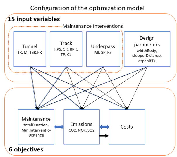
Figure 1 variables of the optimization
The fifteen maintenance interventions are supplemented with three design parameters as the input variables in this model. Because of the added complexity by considering more maintenance interventions and design aspects the genetic algorithm needs more evolutionary stages to come to a sound solution space. At the same time it is important to keep in mind that with too much iterations a genetic algorithm can reach a problematic stage of overfitting where a solution is optimized to much to the evaluated data that it is not applicable to situations with slight changes in the data. Then the obtained results are useless. The following depicted results were obtained with the nsga2 algorithm on a population size of 100 per generation and 30 generations.
Pareto front of total duration of inventions as a function of the costs
Here the total duration of interventions is shown as a function of the costs. The blue line represents the pareto frontier. At the left edge of the diagram one can see that even when you completely disregard the duration of interventions there is a certain amount of costs you cannot undercut. Moving to the right, with higher costs you can reach situations with lower duration for maintenance tasks. But intuitively at some point you cannot buy a faster duration and this trade-off stops. Further to the right we can see that a higher total duration even results in higher costs. While that seems counter-intuitively as a solution on the pareto front, be reminded, that only two of the six objectives are depicted in this diagram. Every point that is pareto optimal regarding all six objectives lies on the frontier. Pareto optimality is a state were the system is optimized in a way that one dimension (objective) cannot improve without a second dimension worsening.
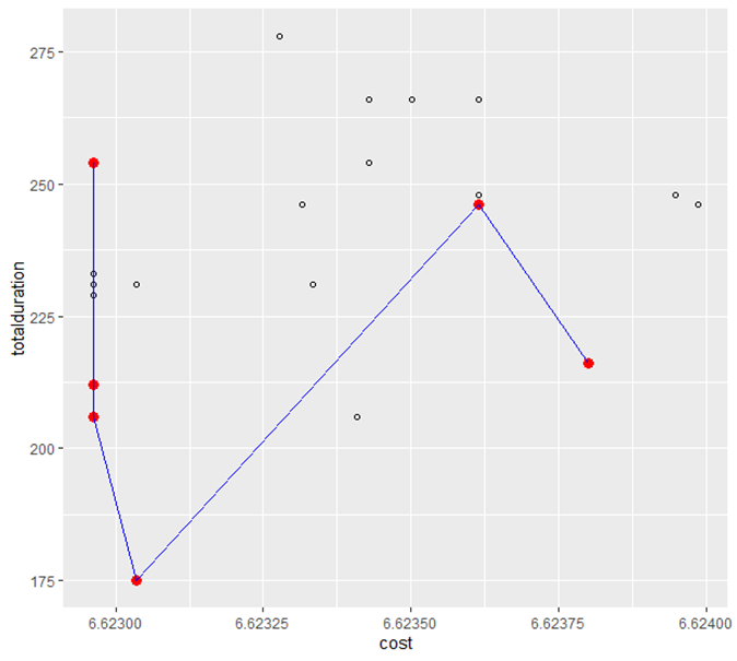
Figure 2 Pareto Frontier – Duration to Costs.
Pareto front of minimum intervention distance as a function of costs
When looking at the intervention distance as a function of the costs one can see that the most frequent solution has two years distance. On earlier evolutionary stages only solutions with one year distance were found. The solution with the maximum minimal intervention distance has a distance of five years and because it is the best solution in that dimension it is inevitable pareto optimal.
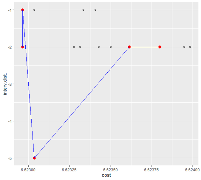
Figure 3 Pareto frontier – intervention distance to costs
Impact of input Variables
Figure 4 represents with the red lines every solution that is pareto optimal and with the smaller blue lines additional non-optimal solutions. There is a lot information inherent in this graphic, as it contains the input variables on the left side as well as the objectives on the right side. Now follows a fine selection of relations revealed by this graphic:
- In column int.dist one can see that most of the pareto optimal solutions have a minimum distance between interventions of two years, sustaining the insights gained in figure 3.
- The sleeper distance is almost always chosen as large as possible to save material and thereby emissions and costs.
- When resurfacing the underpass, the upper bound is never exhausted or even remotely reached. The underpass is resurfaced much earlier than technically necessary.
- The opposite is the case for the cleaning of the track. There, the lower bound is never reached and the cleaning is done on the rarer side of the possible spectrum.
- The solution with a low total duration and five years min. intervention distance seems to be associated with a very high NOx load.
- Especially the bounds of the interventions where all pareto optimal solutions are on the edge should be looked at again. A basic rule of optimization is that the binding constraints need to rely on the most solid data. Because a slight change in this bound will directly change the outcome, in contrast to non-binding bounds. A sensitivity analysis could provide insights which binding constraint influences the objectives the most.
There are many more observations to be made. What did you find out?
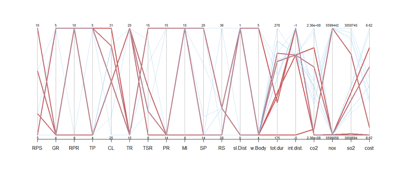
Figure 4 Connections between the variables
For a more detailed look in Figure 5 and 6 the graphic from above is divided into input and output variables. Please keep in mind that thereby also the connection which pareto-optimal input combination corresponds to which output combination is severed.
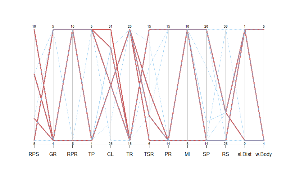
Figure 5 Characteristics of the input variables
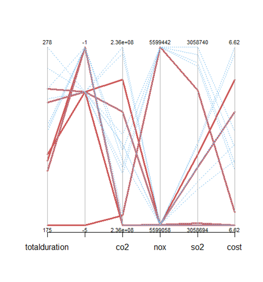
Figure 6 Characteristics of the output variables