In our project, we have 4 different systems: Bridge, railway track, retaining wall and cable car. Normally, these systems contain different maintenance events and the durations of these maintenance events are also different. In order to ensure maximum efficiency for users, maintenance works must be organized under certain obactive functions. These functions are, maximizing the time between interventions and minimizing the time the system is not in use due to the interventions. When considering the context in which we connect these systems, one of the most important points that we paid attention is the operation of the other option if one option breaks down in a transportation network that carries travelers from point A to point B. For this reason, we made 2 groups out of the 4 systems we have. Bridge and railway track were analyzed as one group, and retaining wall and cable car as another group. Thus, the cable car can be used while the bridge and track are in maintenance.

First, interventions and frequencies of interventions are considered independetly to calculate the total duration of intervention and result is obtained as 226 days. Following sketches show how these interventions are scheduled.

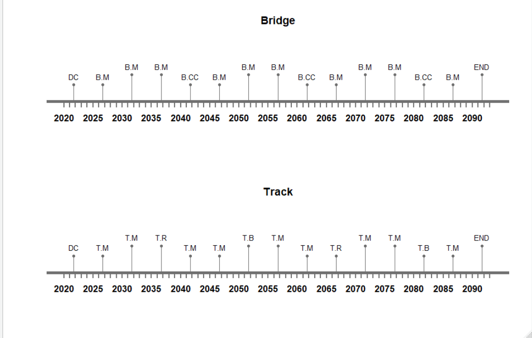
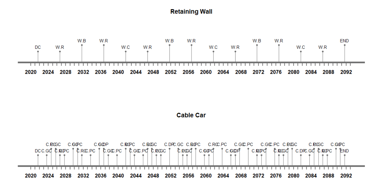
Figure 1: Intervention schedule for independent interventions

 If the interventions in the same group start together and conducted with same frequencies. Intervention duration drops from 226 days to 200 days. For this strategy, following schedule is obtained.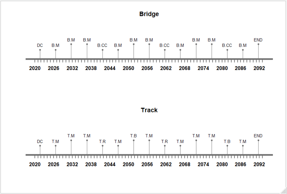

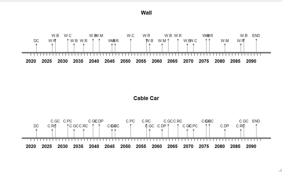
Figure 2: Intervention schedule simultaneous interventions

To find the optimum intervention schedule, following frequency ranges are defined in each pairs

1st group:

events.grid.bridge <- expand.grid(B.CC = sample(seq(17,24, by = 1), n.grid),
B.M = sample(seq(2,9,1), n.grid))
events.grid.track <- expand.grid(T.R = sample(seq(12,18, by = 1), n.grid),
T.M = sample(seq(2,9,1), n.grid),
T.B = sample(seq(25,35,1),n.grid))

2nd group

events.grid.wall <- expand.grid(W.B = sample(seq(7,13, by = 1), n.grid),
W.C = sample(seq(16,24,1), n.grid)
events.grid.cablecar <- expand.grid(C.GC = sample(seq(1,7, by = 1), n.grid),
C.PC = sample(seq(1,7,1), n.grid)

After simulations coducted in R, following graphs are obtained.

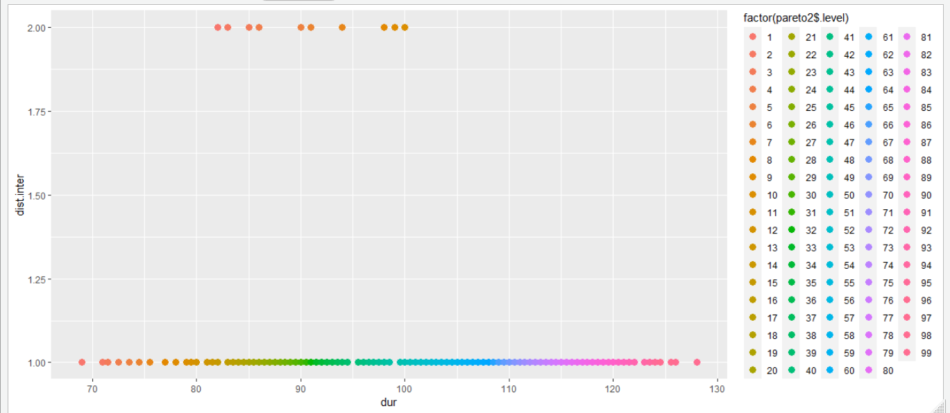
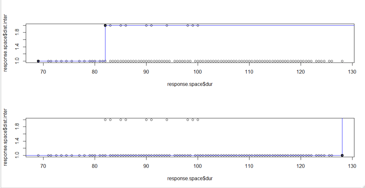
 Figure 3: Pareto fronts for wall-cablecar

The blue lines in last two graphs show pareto frontiers based of different predefined preferences for the group of wall and cable car system. First graph aimed for low intervention duration and the other one aimed for maximizing time between interventions. Among almost 130 found alternatives, dark blue point shows the best alternative for the defined preferences.

Following graphs are obtained for the bridge-railway track group.

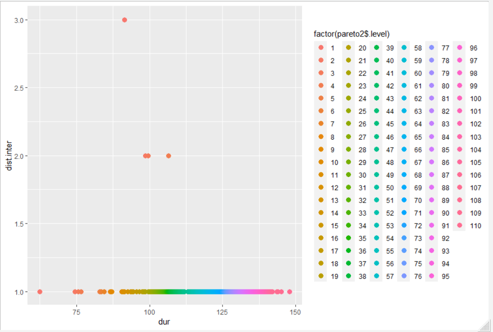
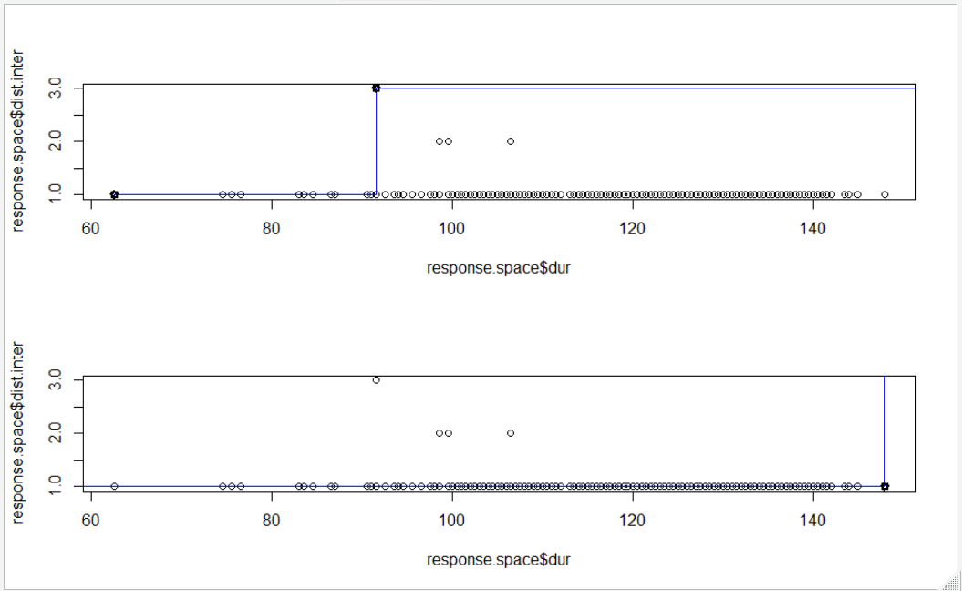
Figure 4: Pareto fronts for birdge-railway track