Multi-objective optimization models are necessary for decision-making processes within complex systems and projects to make decisions more transparent according to the considered criteria. Different multi-objective objects are combined within defined variation intervals over an observation period and applied to specific project-specific objectives of the individual multi-objective objects. A genetic algorithm is used for this purpose. The results of these investigations are used to show the dependencies (relationships) of the observed variables (multi-target objects) from the data. The essential tool for this is the use of Pareto fronts. A Pareto front represents a type of trade-off solution simulation in which a change in value (improvement) of one of the multi-target objects would lead to a deterioration of another object (criterion). Based on the results, the project stakeholders can make their decisions for the multi-objective problem based on the best possible solution paths of one criterion, while being aware of the impact on the other project parameters (other multi-objective objects).
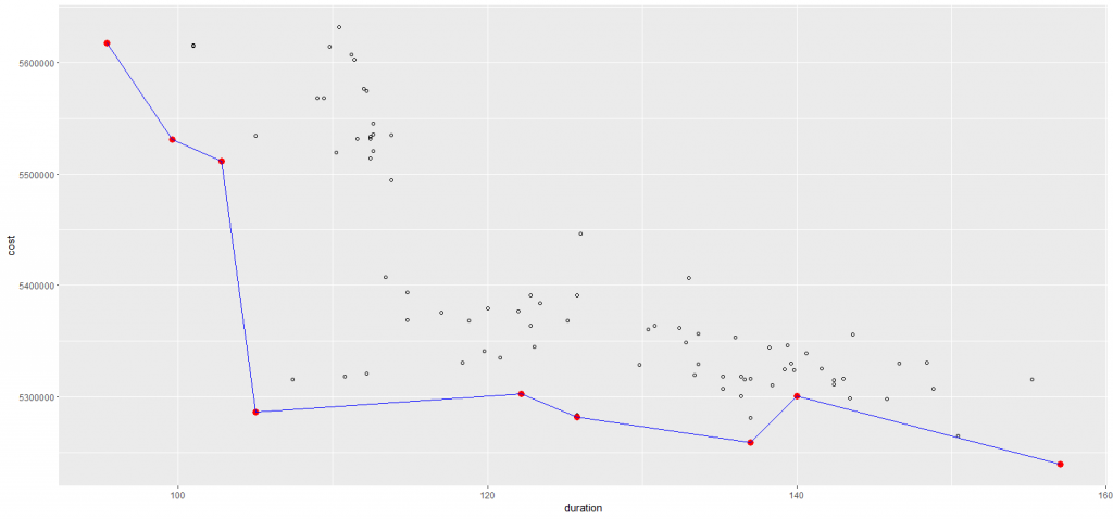
Using the results of our first plot (Figure 1), we can evaluate the Pareto solutions of the genetic algorithm for minimizing the duration and maximizing the distance between two interventions. The results are presented graphically in a plot of cost and duration. The red points are the Pareto solutions. Based on several runs of this simulation, it can be seen that the Pareto fronts are very different. Therefore, the significance of the Popsize and Generation variable can be determined. These are on the one hand responsible for the run size of the population of the algorithm, thus the diversity of the scenarios and the number of runs of the algorithm, thus the quality of the Pareto solutions. Accordingly, the diversity of the result plots is a measure of the accuracy of the solution to the problem under study. The calculated costs of the solutions can be compared with the previously desired project goals. If necessary, an increase in the variables of the GA can be made based on the results of the duration and dist.intervention. A consideration concerning the Value of Information for the investment in computing power should be made in advance. What the algorithm does is try out different combinations of our input variables, regarding their boundaries, than compare the outcomes, trying to minimize them and looking for the Pareto front. It is clear, that the more combinations you try, the better results you get.
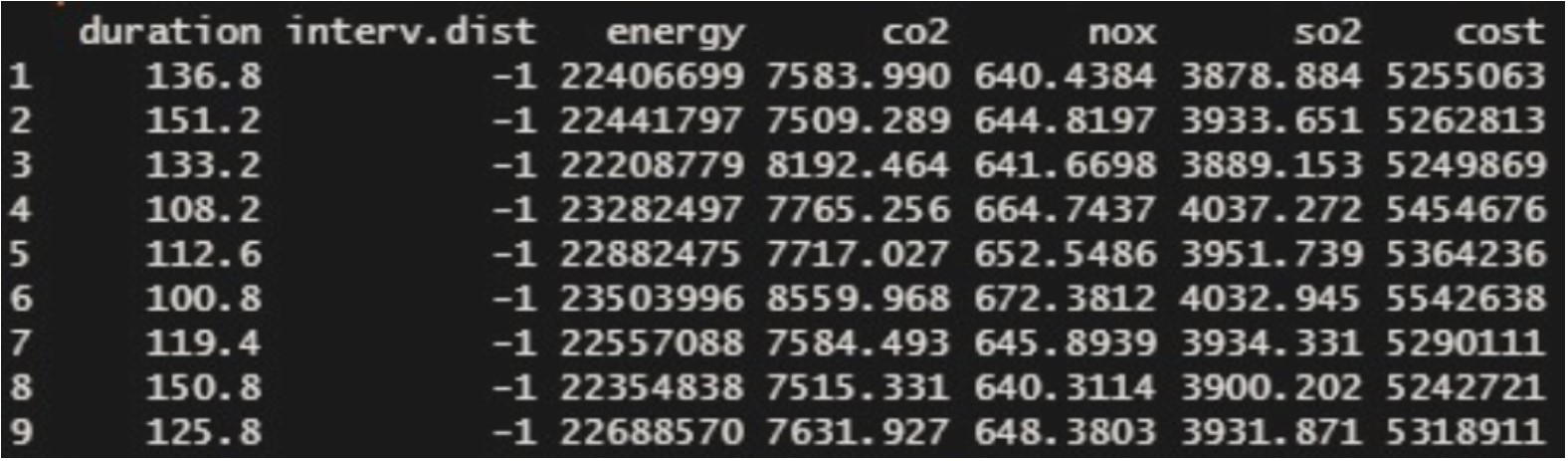
To understand the influence of the initial values of the algorithm, the accumulated values parameters are presented. Therefore, in the plot (figure 2) all interventions are listed side by side along with the entries of the result vector. Our results vector represents the results in 7 different criteria. The first entry represents the total duration of the interventions. The second entry shows the minimum intervention intervals. Entries 3 through 7 present the summed values of emissions and associated costs resulting from the combined maintenance scenario for the entire system.
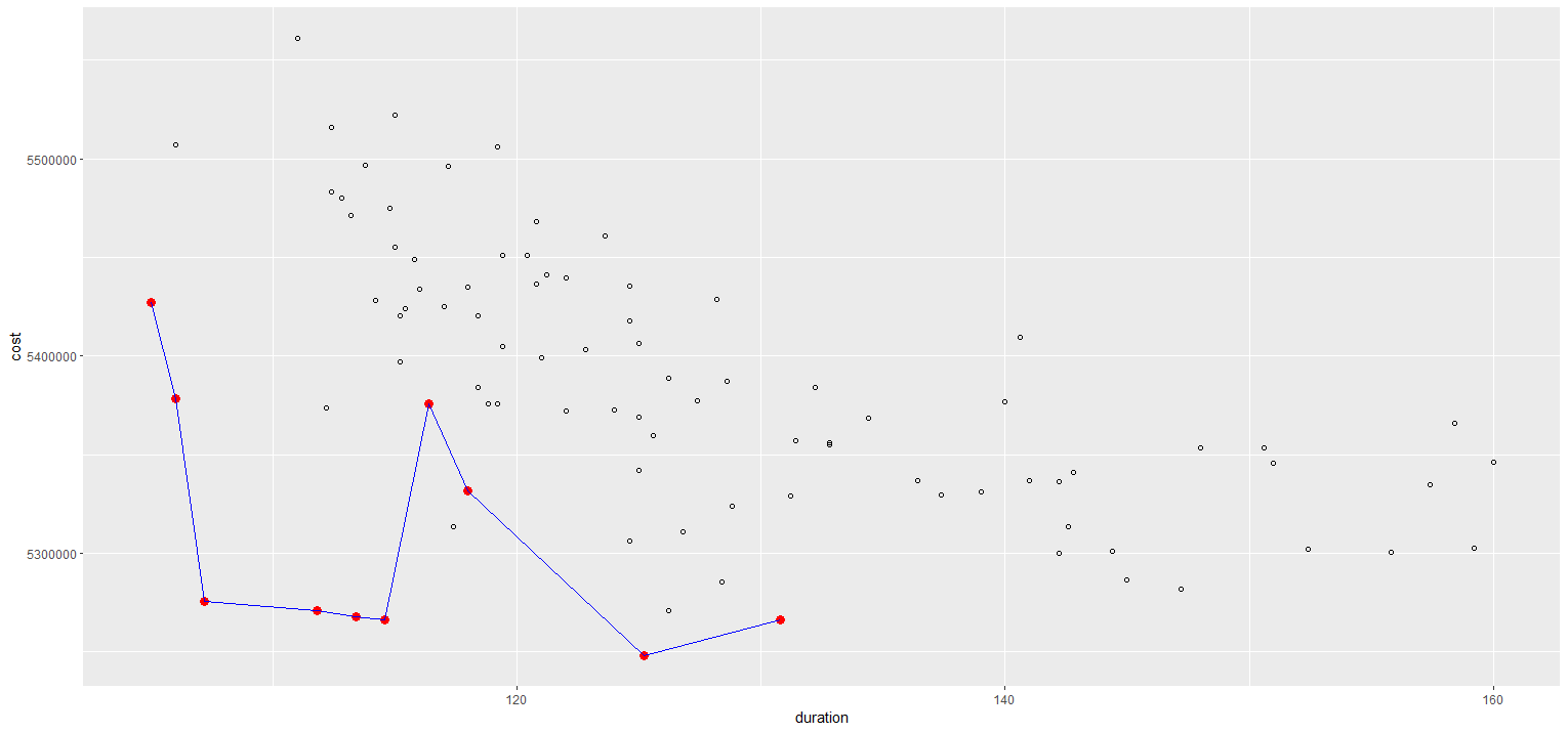
Based on the previously defined targets for the duration and minimum intervention time, the Pareto fronts (red lines; blue = suboptimal solutions) are visualized accordingly. From this, it can be seen what influence the respective Pareto front has on one of the other parameters. Based on these data, a decision can be made for the 2 selected targets. Subsequently, based on the Pareto lines, a decision can be made about the other secondary targets, in this case, the reduction of emissions and also of costs. Thus, from these results, there is the possibility to make a trade-off between benefit-oriented system goals, economic efficiency as well as sustainability. In order to apply these results comprehensively to the project or to integrate only a few additional parameters for the decision-making process, the individual results must be weighted in an AHP analysis, for example. Nevertheless, these analyses are the data basis for decision-making of complex system operations or projects.
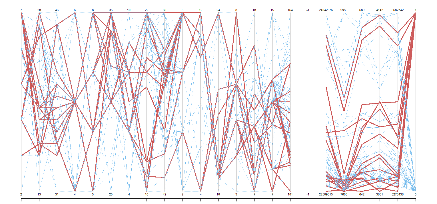
In Figure 3 you can see the numbers the algorithm tried and which were leading to the Pareto results. To give an example, the first maintenance plan which is Pareto optimal would be to have p.1 every 6 years, p.2 every 25 years, p.3 every 38 years, w.1 every 4 years etc.
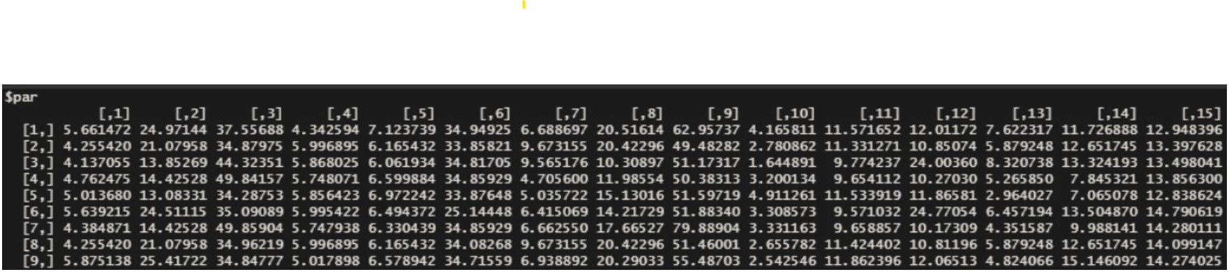
This maintenance plan would then lead to the following outcome in duration and related costs to energy and emissions (figure 4). Our example before would lead to a duration of 136.8 days, and costs of, 5255063 €.
Conclusions:
From the investigations carried out for the maintenance planning of complex systems, we were able to determine the significance of the relations between individual subsystems. Thus, the importance of the reliability of an individual subsystem in the context of the overall system became apparent. In the course of the combined maintenance planning of the entire system, we were able to increase system reliability and thus usability by defining specific goals for the results’ strategy. In the life cycle analysis, it became clear what influence the maintenance measures have on the project costs and emissions. Therefore, it is important that maintenance measures are minimized by bundling and preventive concepts are created to avoid large costly measures. Different simulation methods were applied to determine a reasonable frame for the effort of computing power with the associated costs and the obtained results for the real application in the scope of the project.
Understanding how cost-intensive maintenance can be, this analysis should also motivate to plan systems as resilient as possible and of high quality. This will maybe lead to higher initial costs but can save costs during its lifetime, regarding that these systems will need less maintenance.
Another prospect for further analysis could be to implement the assumption, that some seasons of the year are more adequate for maintenance on certain systems than other seasons. In our system, it would for example make more sense to have these interventions during the summer, when there is not as much energy required for heating the households.