After combining all four lifetimes, a total duration of interventions of 185,5 days during the set lifetime of 50 years were computed. This means that there is a relatively low overlap of maintenance strategies of the individual systems.
Succeeding, more possible scenarios through the simulation of all attainable outlines of each system with an output of the total duration of interruption were implemented. These were realized with a set grid of two, which means that two values were extracted from each range of frequency defined for each individual system. The following list display possible results for each individual system.
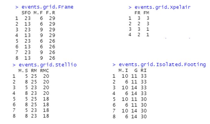
The preference of the simulation outcomes is obviously a minimum duration of intervention and maximum time between the interventions.
Initially our systems were totalizing 185,5 days of maintenance during the lifecycle of the system, which is already more than a semester. So, there is a need to upgrade this value in order to have the maintenances better scheduled (in the best cases overlapping), thus reducing the numbers of days interventions.
To aim this, a Pareto efficiency is done using the frequencies and durations in our scenario space, meaning the set of data extracted from our individual systems as described above (see Fig.2.5). This helps to find the best schedule for planning interventions. Firstly, a combination is made with regards to “lowest intervention durations and high time gap” between the interventions. Fig.2.6 shows the results obtained by this configuration.
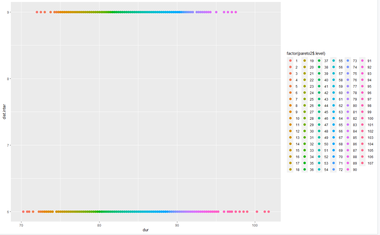
The results can already be evaluated by the visualized color index: The orange color displays the best solutions and the pink being the less suitable. But the diagram can not be read accurately. Running the pareto frontier enables us to observe the best values for the combination of low intervention durations while maximizing the time between these intervention events.
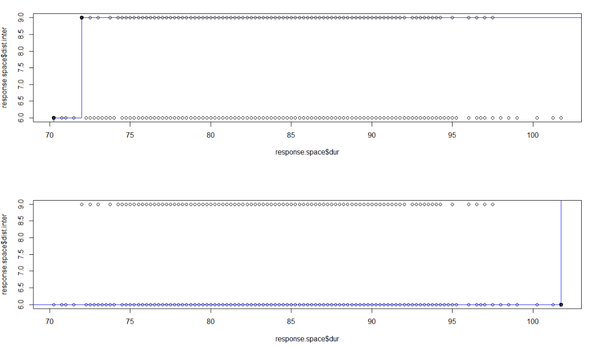
The Pareto frontier display that maintenance days revolve at around 70 days for the best solution and even the worst solution still targets around 100 days of maintenance. The table below shows the numerical values for the interventions in the two most suitable solutions described above.
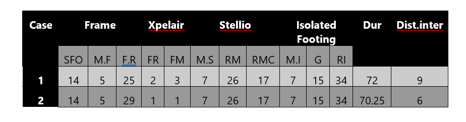
Concluding, the first solution accounts a little more maintenance days with 72 day compared to 70.25 days for the second solution. But the time between the interventions is higher for the first solution with 9 years compared to 6 years for the second solution.
During a Multi-Objective Optimization, an optimization of these maintenance strategy will be done to improve these discussed values.
Page Navigation
2.1 Maintenance Strategy of Individual Systems
2.2 Integrated Maintenance Strategy
3. Life-Cycle Inventory Analysis