The main goal of this Multi-Objective Optimization (MOO) is to combine individual systems with each other by combining their maintenance plans over a lifetime of 50 years. In the course of the integration context the optimization will lead to a minimization of costs while causing a maximization of functionality time. In detail, the aim is to maximize the time between the interventions while minimizing the total number of interventions as well as their durations (see Fig.1).
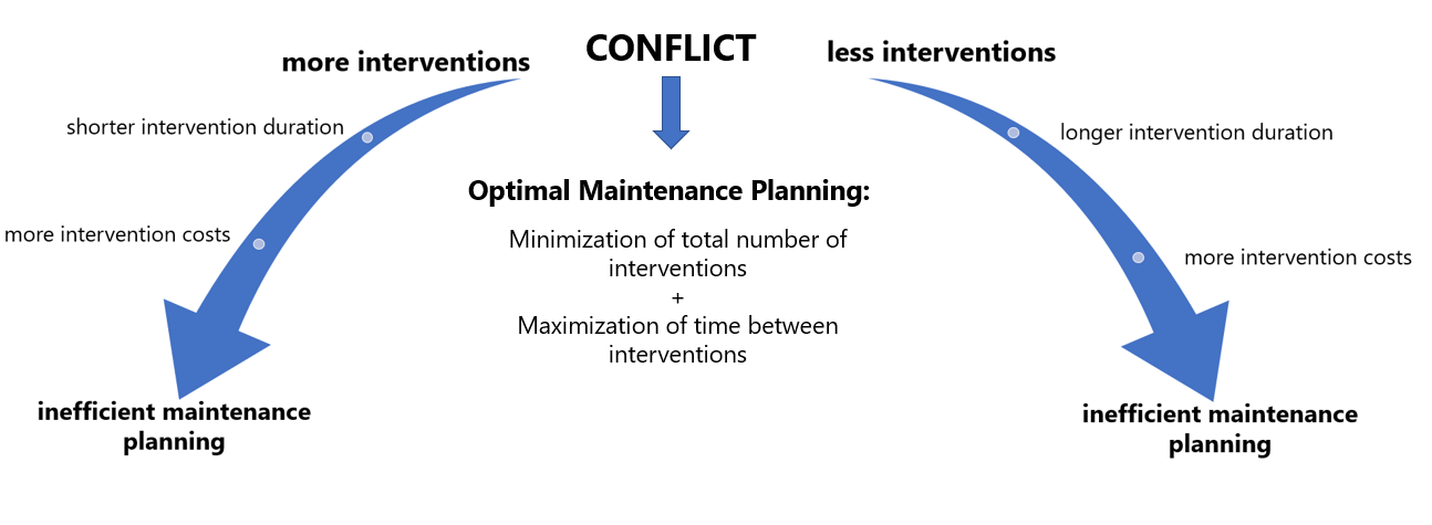
Fig 4.1: Summary of conflicting objectives for the Multi-Objective-Optimization
To satisfy these conflicting objectives a Fitness Function is defined and used as a basis for a genetic algorithm (GA). The GA submits the best set of solutions for the given objectives by using an initial data set provided by the Fitness Function and applies a suitability function to sort out and crossover the data, so that a new data set is generated. These phases are repeated iteratively, until the best data set is found.
The input parameters for the fitness function are defined by a set range of intervention durations for each component as part of the maintenance planning.
- Interventions durations for the Frame
- 13 ≤ SFO ≤ 23
- 3 ≤ M.F ≤ 9
- 25 ≤ F.R ≤ 35
- Intervention durations for the Xpelair
- 1 ≤ FR ≤ 3
- 1 ≤ FM ≤ 3
- Intervention durations for the Stellio
- 3 ≤ M.S ≤ 8
- 20 ≤ RM ≤ 30
- 15 ≤ RMC ≤ 25
- Intervention durations for the Isolated Footing
- 5 ≤ M.I ≤ 11
- 7 ≤ G ≤ 17
- 30 ≤ RI ≤ 40
Moreover, the parameters of width as the integration parameter of the integrated system will be based on a value generated by the genetic algorithm, and thus, also varying within a range.
As the output of the fitness functions the parameters of the total duration, the minimum distance between two consecutive interventions, energy demand as well as the amount of emissions as CO2, NOx, SO2 and their related cost will be derived (see Fig.2). These resulting data set is than displayed in a plot using the Pareto Frontier as the optimal solution.
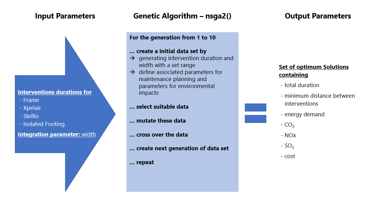
Fig 4.2: Operating Principle of the genetic algorithm applied for the Integrated System
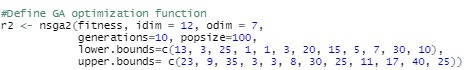
Because of the random character of the GA different results are obtained with every new run of the R-Code as its input parameter are set differently every time. But for each set of input parameters the best solution is found. In R the nsg2()-function is applied for the GA. During 10 iterations (generation) an initial data set consisting of 13 different input parameters (idim) is processed to generate a new data set containing 7 output parameters (odim) out of 100 alternatives (popsize).
Fig 4.3: Application of the nsg2()-function with defining lower and upper boundaries for the generation of the data set
Because of the random character of the GA different results are obtained with every new run of the R-Code as its input parameter are set differently every time. But for each set of input parameters the best solution is found. In R the nsg2()-function is applied for the GA (see Fig.3). During 10 iterations (generation) an initial data set consisting of 13 different input parameters (idim) is processed to generate a new data set containing 7 output parameters (odim) out of 100 alternatives (popsize).
During the Integrated Mainenance Strategy a solution was found for the duration of the maintenance of the integrated system throughout its lifecycle. As a recall, we obtained 2 values, 70.25 days and 72 days, which was already much suitable as the initial duration of 185 days. Similarly, we obtained of the Life-Cycle Analysis the results for the combined system, containing the energy consumed by the individual systems and the emitted greenhouse gases (CO2, SO2, NOX) as well as including repairs till the end of the system’s lifecycle.
In order to improve the maintenance strategy the maintenance period and/or the costs involved in the lifecycle will be reduced. For this aim, a pareto front is being expressed graphically to explore these alternatives. A total of 12 alternatives are generated and are shown in the diagram below (see Fig.4.4).
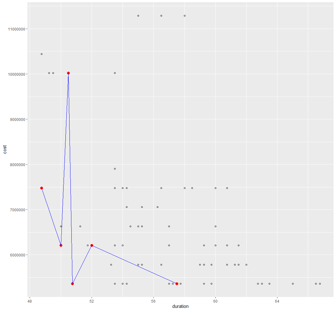
From these alternatives, it is possible to figure out 2 options: The least costly (costs in Euros) and the one with the least duration of maintenance (duration in days). They are shown in detail on the table below (see Fig.4.5).

By this, it gets obsious, that the optimization does reduce the maintenance days by 30%, which is a great improvement. From these options, a conclusion could already be made, if the stakeholders only stick to those two factors (time and money). Still, they are not the only objectives, so that for each of the 12 solutions other factors (emissions, energy and interventions) should be taken into consideration. The values of all factors included in the option are shown in the diagram below (see Fig.4.6).
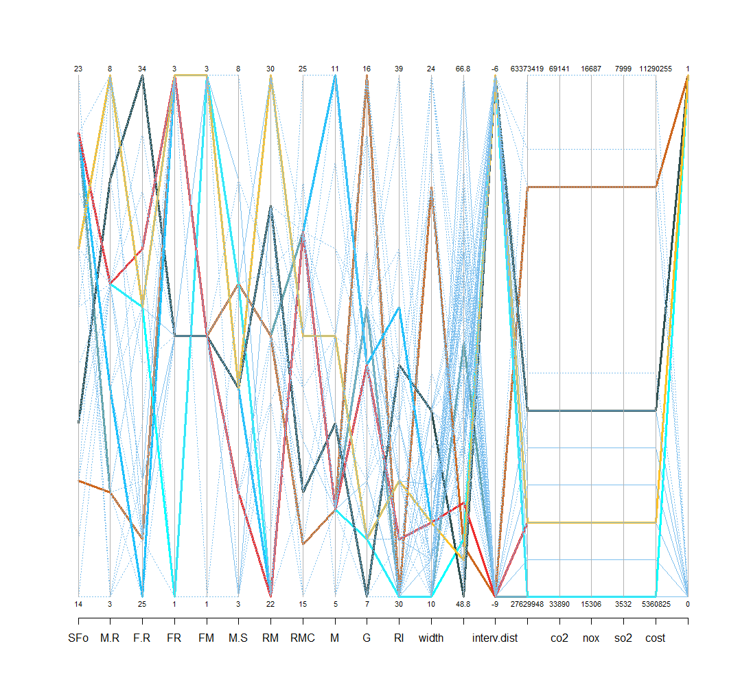
Each option is visualized with a color (alice blue, azure, blue, cadet blue, chocolate, cyan, dark grey, dark orchid, dark slate gray, deep sky blue, fire brick and golden rod for option 1 to 12 respectively). It can be noticed, that some options consume more energy than others or produce more greenhouse gases than others. These factors may affect the decision of stakeholders depending on the defined scope and goal.
The Interpretation of these data as well as a recommendation for Decision-Making can be found under here.
Page Navigation
3. Life-Cycle Inventory Analysis