Home / Group 2 / Multi objective optimization

Multi objective optimisation

Complex civil systems need optimised maintenance strategies in order for them to last the intended lifetime, to minimise their cost and to decrease the systems down time. In order to do this, we must accurately model the system including the stresses and maintenances the system undergoes in its lifetime. In this assignment we do so with the help of multi objective optimisation.

The main criteria we considered when optimising the maintenance strategy are the following:

• Maximise the time between interventions
• Minimise the time that a system is out of use.

Multi objective optimization generalization implements the use of a genetic algorithm. For that nsga2() function, part of the mco package in R is required. Therefore it requires the function to be minimized, the number of input variables, the numbers of output measures, as well as the lower and upper bounds for the input variables. In order to create the function to be minimized, it is essential to look at the input and output variables. Different maintenance planning strategies need to be analyzed. For this, the durations of the interventions will be considered in a specific range as shown below.

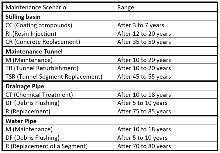
The input variables and the ranges that were considered for these variables were the following:

• Dam length – ranged from 500m to 800m
• Dam height – ranged from 70m to 100m
• Dam width – ranged from 29.24m to 33.34m

Then, another input variables which we will vary within a range is the dam length, dam height, dam width, tunnel length, drainage pipe length, water pipe will be variables depending on the intervention strategies. The output variables will be the total duration of the interventions, the minimum distance between two consecutive interventions, energy, CO2, NOx, SO2, and Costs.Based on this information the fitness function is defined.

 Results for Scenario III

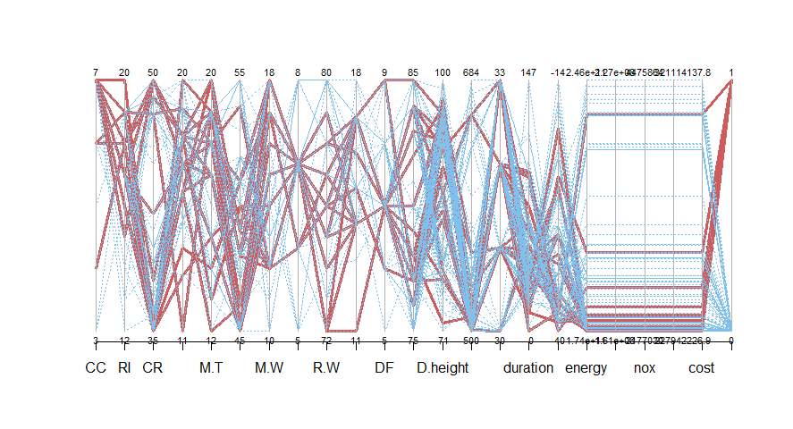
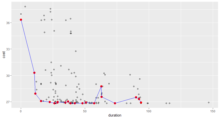
With the help of RStudio the following graphs were generated for Scenario 3. The figure below presents the Pareto frontier of our performance criteria. It considers the time between interventions, the intervention length of each maintenance scenario and the cost of maintenance.

The bottom figure shows the accumulated impact of the input parameters on the performance criteria. Here, the red lines show the optimal solutions, whereas the blue lines show the non-optimal solutions. With regard to the environmental costs, it is fixed for almost all solutions. The reason is that most emissions occur during construction. In contrast, regarding the optimal solution there are ranges for some of the interventions.