With a life cycle analysis, a designer get’s the opportunity to glimpse into the future for possible results of different design decisions. It is not only possible to see what result is created, but also in what way it behaves in relation to different aspects. For example, it is possible to analyze if the increase of costs for growing systems also grows in proportion or if the change is different.
To conduct the analysis for the combined system we create three different LCA-functions named after the parts they are used for (pipe, beam and wall). Each function at the start calculates the effective weight for the system which is used for the cost calculation of the associated system.
By using the Life-Cycle inventory the emission values from it are multiplied with the weight to get the emission costs. With the maintenance data, consisting of maintenance types, durations, frequencies and costs, the maintenance costs for the system can be calculated. Due to the addition of an additional “maintenance postponement”-factor, the costs of each maintenance action increase by 10% for each year of maintenance postponement with the assumption that each maintenance is harder or more expensive with components in worse conditions.
After establishing the weight factors for the Life-Cycle data and the system parameters, the LCA’s of each system can be calculated. The LCA functions can also be combined for the calculation of the integrated system. Results for the current system parameters are shown in (Figure 1):
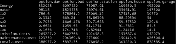
Figure 1 LCA results of each system
The results show that the parking house with the garage as the observed system has the highest overall costs for the chosen system parameters. To analyze if the results are the same for different parameters, a step scaling Life-Cycle analysis was introduced.
In the step scaling analysis, a control variable “f”, ranging from 0 to 1, is introduced which is used to scale system parameters evenly. By using system design parameter ranges with minimum and maximum values the control variable determines which parameter value is used. For f=0 the minimum value of the parameter will be used while for f=1 the maximum value from the range is chosen, with every other value between the range being used for other “f” values. The internal calculation of the values is done by determining a delta or ratio, describing the difference between minimum and maximum value of both considered design parameter dimensions, and multiplying it with the current control variable “f”.
After calculating each scaled value for all systems, the results are saved in a matrix containing all the cost data. The evaluation results of the scaling step analysis are shown in (Figure 2, Figure 3, Figure 4 and Figure 5):
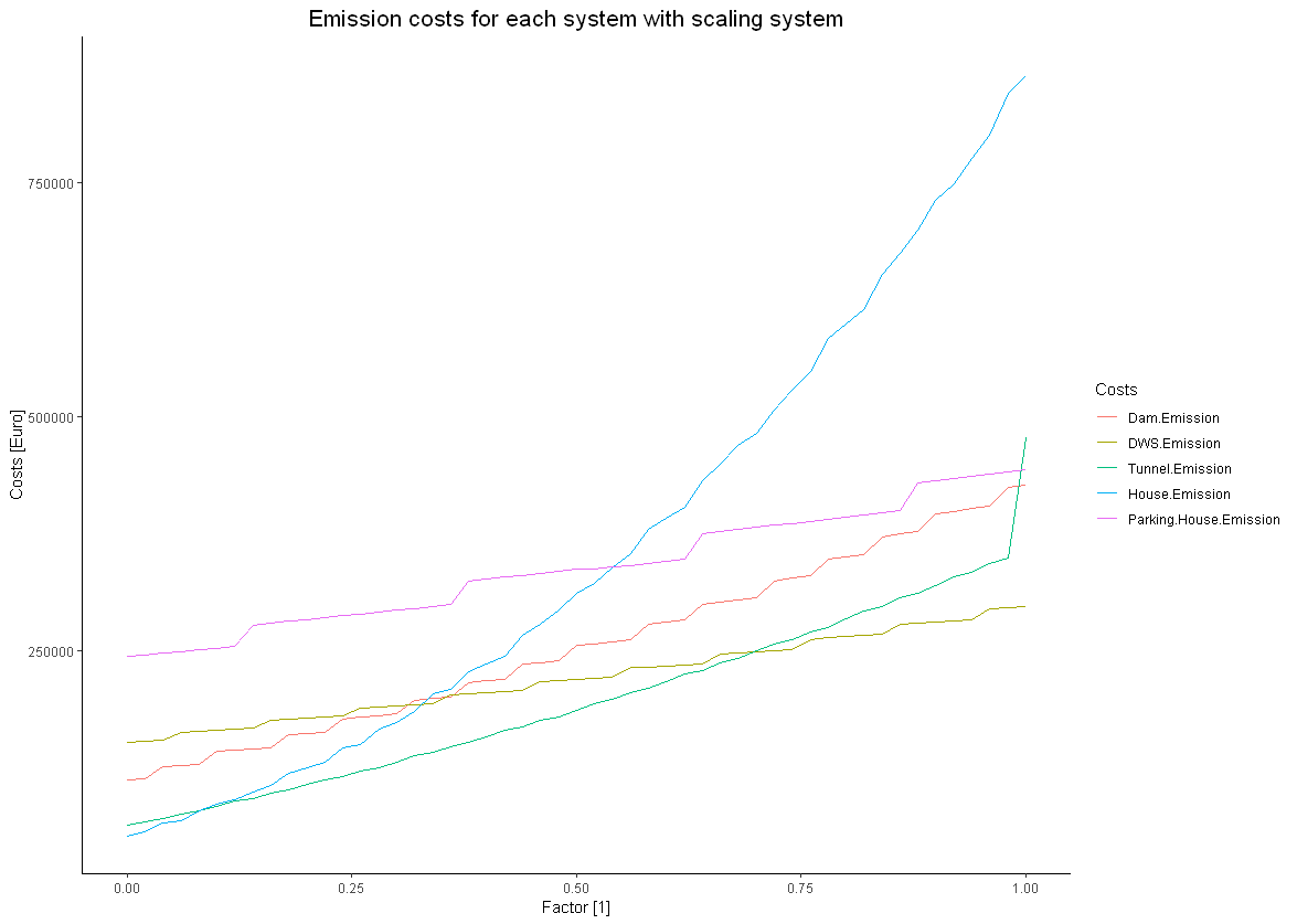
Figure 2 Emission costs for each system in relation to the control variable
The results show that the emission costs for the parking house are by far the highest when the minimum values of the system parameters are used. On the other hand, the house emission costs are growing exponentially and are already the most expensive at a scaling factor value of a bit over 0.5 where the system parameters are in the middle between minimum and maximum value. While most system growth behavior is linear overall, the house system shows a different result. All systems have in common that after a set amount of parameter increase a jump in costs occur. This can be explained by the use of the rounding equation in the calculations. Without the rounding, the continuity of the graphs would be more apparent.
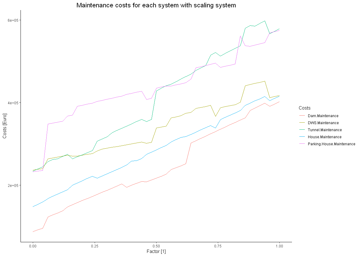
Figure 3 Maintenance costs for each system in relation to the control variable
The results for the maintenance costs look more erratic than the emission graph. This can be explained by the change of maintenance frequency and the associated best solutions for it. The garage system stays as one of the more expensive endeavors over the whole scaling range with the tunnel system overtaking it in cost maximum after half the range of the control variable. Even though the gradient of the garage system is less high than the other systems the high initial costs make sure that this system is the most expensive one in all parameter ranges. This result can be used for priority checks and planning processes.
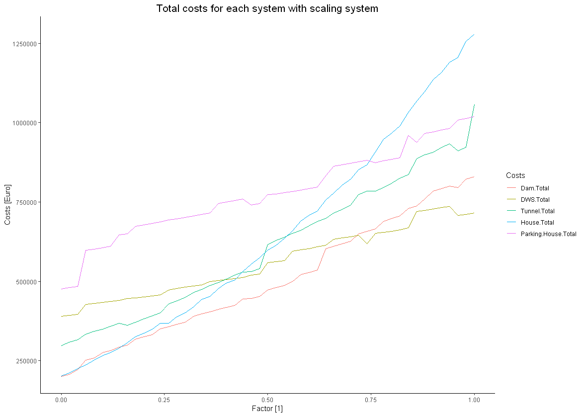
Figure 4 Total costs for each system in relation to the control variable
The total costs of all systems have one trait in common: the graphs take the distribution form of the costs range that is more expensive. While most system graphs take the distribution of the maintenance cost, the house system graph looks similar to the emission cost graph.
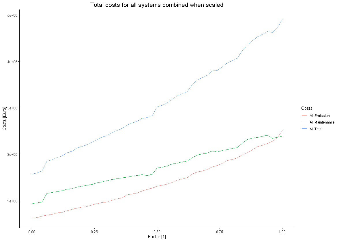
Figure 5 Cost distribution of the combined system
The combined results of the cost distributions show similar results the other ones. On thing to note is the impact of the house emission costs with its exponential growth resulting in total overall costs that are also exponential to the scaling factor resulting in rising cost increments that are economically not desirable.