Risk-based assessment of systems condition
A flexible pavement structure generally comprises several layers of materials that can accommodate this “flexing”. Roads are areas of asphalt that “bend” or “deflect” due to traffic loads, making them less susceptible to damage and requiring fewer repairs over time. Each layer receives loads from the above layer, spreads them out, and passes on these loads to the next layer below. Thus the stresses will be reduced, which are maximum at the top layer and minimum at the top of the subgrade. High flexural strength. The strength of the road is less dependent on the power of the subgrade. Low ability to expand and contract with temperature and therefore need expansion joints. High ability to bridge imperfections in the subgrade. Essentially, flexible pavement is more adaptable to the elements to which it’s exposed. The initial cost of mixing and applying flexible pavement is low and with excellent regular maintenance, it has a lifespan of about 10-15 years. Based on real-life data based on the monitoring of the pavements, let’s assume that at the time t, we have no.t =250 flexible pavements with a condition rating of “10-9” and at time t+δt from the number of pavements with a rating of “10-9” is only no.delta.t = 213, where δt is one year for pavements. This says us that MTTF for the flexible pavement is 6.7 years; which is the time of reaching the “Poor” state from the “Fair” state. The repair rate μ is dependent on a probability distribution. The new perfect test is shown. If we know for sure that event Q occurs, then we make repairs. In contrast, if we know for sure that the event does not occur, then the asset managers can decide not to make repairs or to delay repairs when the system needs that.
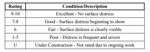
The below table represents the possible states of a Flexible Pavement during its lifetime:
Life Cycle Assessment & Multi-Criteria Decision Making
The goal of this assessment is to conduct a life cycle analysis and MCDA for the sub-system/component of my previous civil engineered product, the ‘Flexible Pavement’. The subsystem chosen for the life cycle analysis and to carry out MCDA is for the two layers of the flexible pavement.
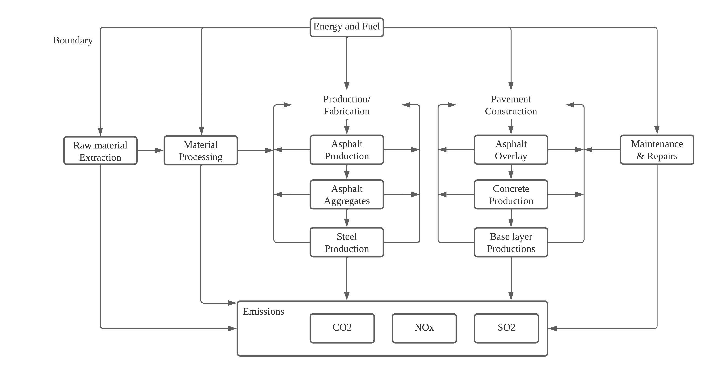
The below figure represents the scope and the boundaries of the assessment:

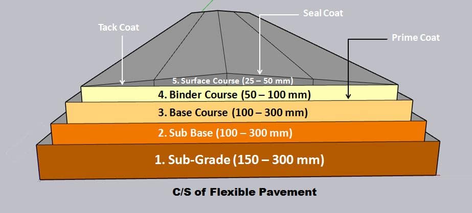
The below figure represents the c/s of the Flexible Pavement:
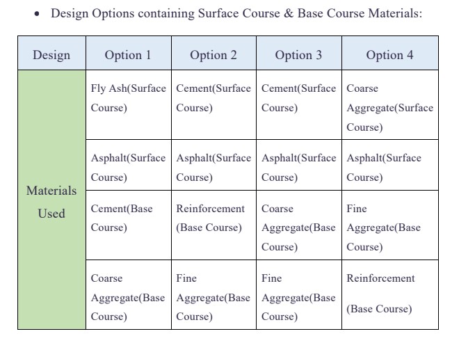 The below table represents the materials used under analysis for the system:
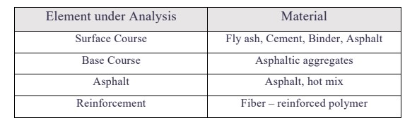
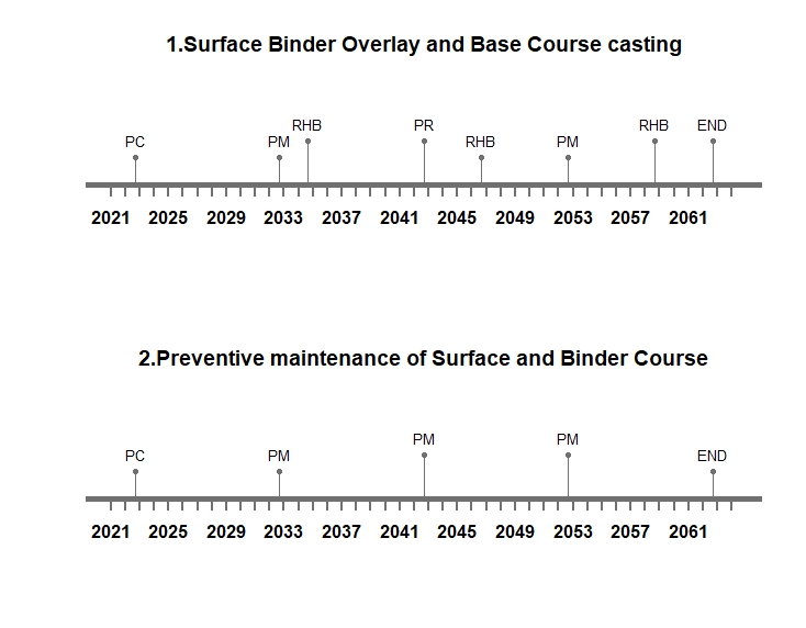
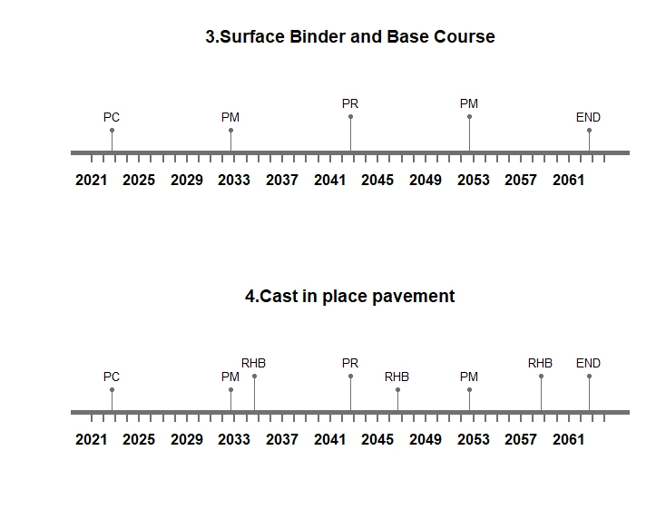
Life Cycle Timeline: As an asset manager, I’ve studied the timeline intensively for the phase: Preventive Maintenance of Surface and Binder Course since it has a recurring intervention of Preventive Maintenance thrice. If we look at the timelines and its interventions, we see that out of all the five interventions, PM (Preventive Maintenance) occurs quite often and the maintenance cost for one intervention is 26707€. For this intervention to occur thrice over a lifespan, the total expense would be 80121€. Preventive maintenance has to be carried out during the years 2033, 2042, and 2053 to fix the pavement and maintain it properly in order to not let it move into other phases or the interventions of the timelines. Similarly, importance should also be given to the intervention RHB (Rehabilitation) since it occurs every 12 years. To be honest, if preventive maintenance is taken care of, there would be no need to give much importance to rehabilitation. In the end, we see that the END of the lifecycle for the flexible pavement is during the year 2063.
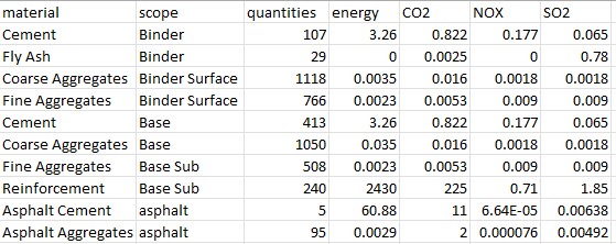
Life Cycle Inventory: The following table presents the composition of different materials used. For each material, the collected information about energy consumption for fabrication and processing (MJ/t), CO2, NOx, SO2 (kg/m3) and cost associated with extraction, processing, manufacture, and construction. The scope column indicates the use of a specific material in the composition of a specific mix, such as Binder and Binder Surface for the Surface Course and Base and Base Sub for the Base Course. For asphalt, the values indicated represent percentages of various materials used in 1 cubic meter of asphalt, such as 5% asphalt cement and 95% aggregate.
The blow table depicts the Life Cycle Inventory of different materials, performance, and environmental indicators:
The bar plots were obtained as follows:
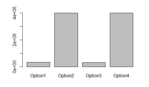
Energy Consumption for different design options
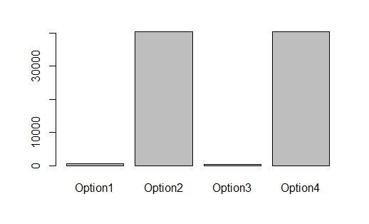
CO2 emissions for different design options
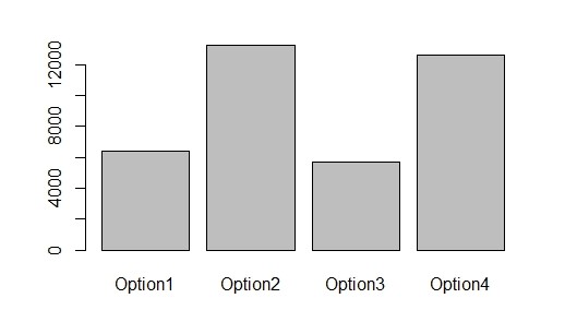
NOx emissions for different design options
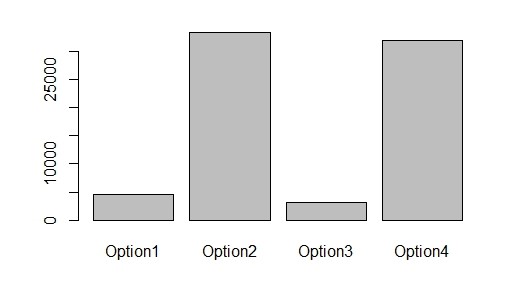
SO2 emissions for different design options
Radar Plot:
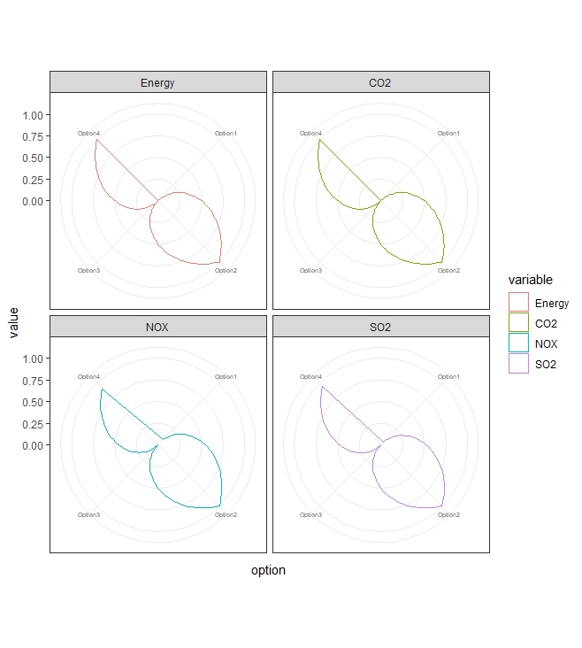
From the above bar charts, we can easily point out that there is less consumption of energy in Option 1 & Option 3; along with lesser GHG emissions produced compared to Option 2 & Option 4. Hence, Options 2 & 4 can be ruled out. By comparing Options 1 & 3, with detailed observations, the energy consumed and the CO2 emissions during the whole life cycle are almost the same. Moving onto NOx emissions, the minimum emission of 5900 kg/m3 is considerably seen in Option 3 than in Option 1. Finally, the least SO2 emission of 250 kg/m3 is attained in Option 3. Since the energy consumption & the CO2 emissions are considered the same in these two options, it is slightly difficult to make a decision considering which option would be the best for implementation purposes. Hence, this decision can be made using MCDA which is the next step in this assignment.
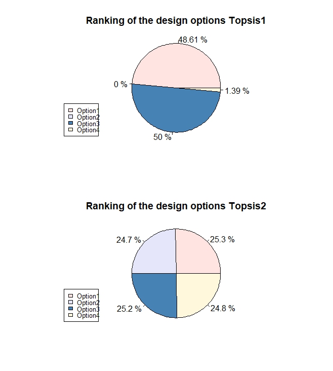
Multi-Criteria Decision Analysis (TOPSIS): TOPSIS method works based on the comparison of positive and negative ideal solutions. The first pie chart represents the comparison of solutions with normal idealised values and the next pie chart represents the same but shows a detailed view of the percentile of the different options to be considered for the execution/implementation of the decision for the project execution. Hence we can say that Option 1 is most likely to be considered for project execution purposes.
Other Systems: