Importance:
Maintenance plans are important for prolonging the lifetime of any project. The need for maintenance plans is to provide corrective measures or preventive measures which will either improve state of the project if it is deteriorating or slow down the deterioration process. For this reason, maintenance planning is executed in every civil system. Apart from lifetime of the system, conducting maintenance will reduce unexpected breakdown of the system.
Looking in depth of the importance of maintenance planning is that we can configure inefficiencies in the system. Once a system is working in full capacity, profits can be maximized. With scheduled maintenance, we can have optimization of resources and assets based on the priorities that precedes. This way, we can target areas that affects the overall system or the built environment the most. Inspections and maintenance at regular intervals can help nullify the probability of any risk or hazard which would provide safety to all the stakeholders involved. With timely repairs and maintenance, the reliability analysis of the system would show good results. If maintenance is executed the way planned, it will promote sustainability and user/client satisfaction.
Strategies of Individual Systems:
Strategies for maintenance matter as they will define the amount of resources to be utilized over the lifetime of the system. It will also affect the energy consumption and output given by the system for its whole life cycle.
Maintenance strategies start by establishing a clear goal for the assessment which should be aligned with the objective of the system. Boundary conditions is also an important element, in our case it will be the whole life cycle of the system. After establishing this, we will need to see the combinations of the design options which will aid us in deciding the types of maintenance and repairs we will have to execute. Depending upon the resources available and reliability of the design options we can determine the frequency of the interventions and the type of maintenance to be used.
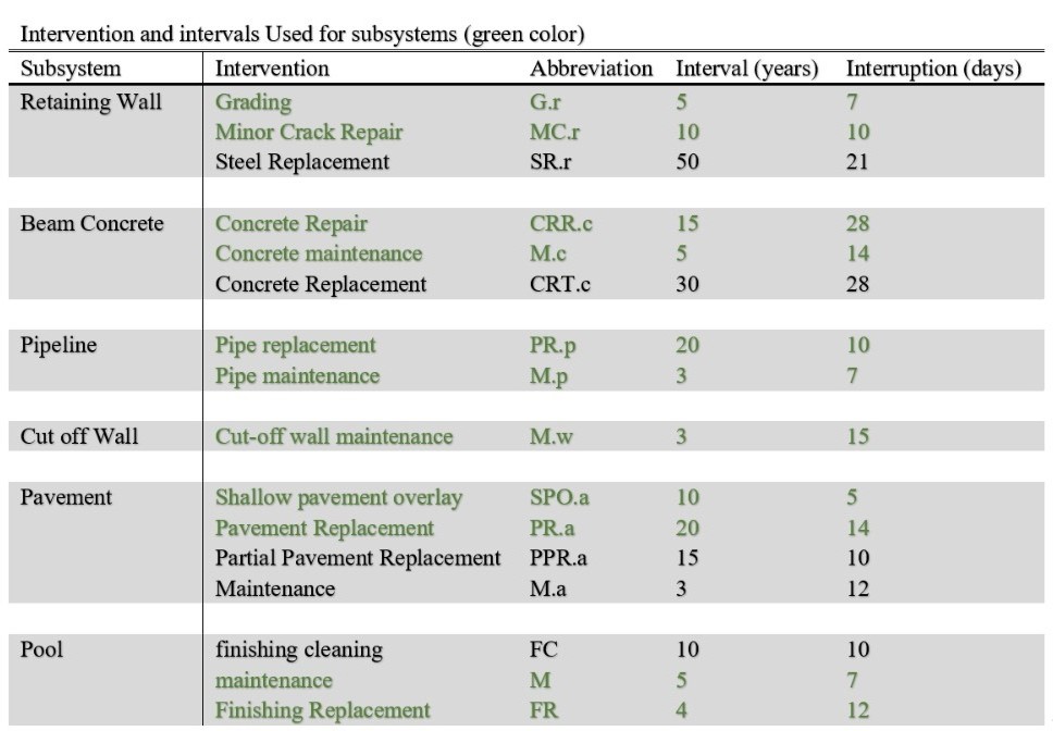
Fig 1 : Interventions Table for Individual Systems
Below is the table for the lifespan of all the individual systems integrated in this project.
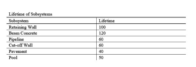
Fig 2 : Lifetime of Subsystems Table
More details about the sub-systems maintenance strategies can be found in the individual systems.
Strategies of Integrated System:
To bring the uniformity to the individual system, the calculations were based off the total lifespan for all systems to be 60 years. The lifetime of the most integral part of the project, the pipelines and also the cut-off walls.
The purpose of having schedules for integrated system rather than the individual system is to bring a bundled affect on the schedule. When the schedules are aligned, we will be able to find common maintenance days which will reduce the overall downtime of the system. The resource allocation and asset acquiring would also reduce thus we will have reduction in the total cost of the project.
To combine the common maintenance days so that we can decrease the overall downtime or the number of maintenance days. We have assigned ranges of years within which interventions can occur. The ranges are defined keeping in view that the goal of the system is not compromised or the deterioration is not too extreme.
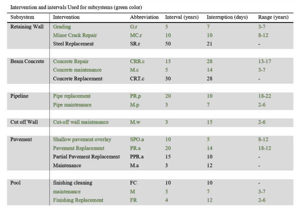
Fig 3: Intervention and Ranges Table of the Subsystems
Individual Timelines of all the Subsystems:
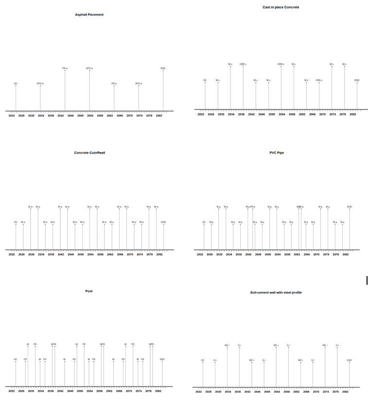
Considering all this information about the lifespan , the intervention and the ranges calculated for the system. The timeline for the 60 years life of the project will look like this.
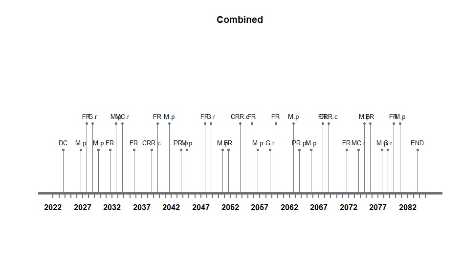
Fig 4 : Timeline of the Integrated System
This information will be useful for planning engineer, procurement officer, inspection team and maintenance team. As the timelines of the sub-systems are in conformity, we will have some common days of maintenance reducing the downtime of the system. All of the mentioned stakeholders can plan out their activities accordingly.
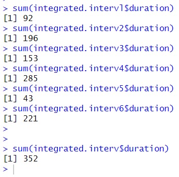
Fig 5 : Sum of Interventions for the sub-systems and the integrated system
The total sum of the intervention days for the sub-systems is calculated to be 990 days based on their individual sum of interventions. Compared that with the sum of interventions for the integrated system, the overlaps due to the ranges and alignment of timelines reduced the downtime to 352 days in the span of 60 years. The maintenance strategies are same and frequency is also same but the common number of days are taken together. Thus, we have more days when the system will be operational.
Now, we have to narrow down the ranges of the interventions so that we can get the optimized maintenance schedule. To get the optimized schedule, we will need to use low function to calculate the minimum duration for interruptions and the high function to determine the maximum distance between two interruptions. In the R-script, we will make to two matrices for each sub-systems. One for the design options of the sub-systems and the other for the maintenance scenarios as defined earlier.
![]()
Fig 6 : Lifetime Scenarios
The lifetime scenarios for the 6 sub-systems combined together for the ranges and design options established earlier is 4096 combination. By perform the analysis with n.grid at 2, the duration of interventions was deviating by +/- 2 and the distance between two intervention was deviating by +/- 2. This can give a preliminary estimate of the difference that will be made by using any of the lifetime scenarios. Also, we can predict that increasing the parameter n.grid, we can get a more refined deviation. The computing power required could become exhaustive for that. So, this parameter value is also practical.
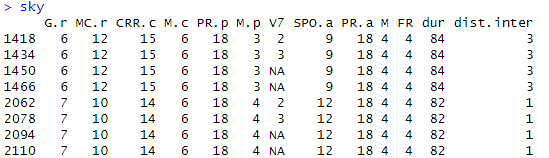
Fig 7 : Top results for low(dur) and high(dist.inter)
Based on the top results, we get 8 different lifetime scenarios. From different maintenance strategies combination, we can either have 84 days of duration for interruptions and 3 years of distance between the interruptions. Or we can have 82 days of duration and 1 year of distance between the interruptions. As we are looking for the combination that optimized by reducing the duration and increasing the distance between the interruptions. We can see that when the duration is decreased we will not be able to attain a high distance between interruptions.
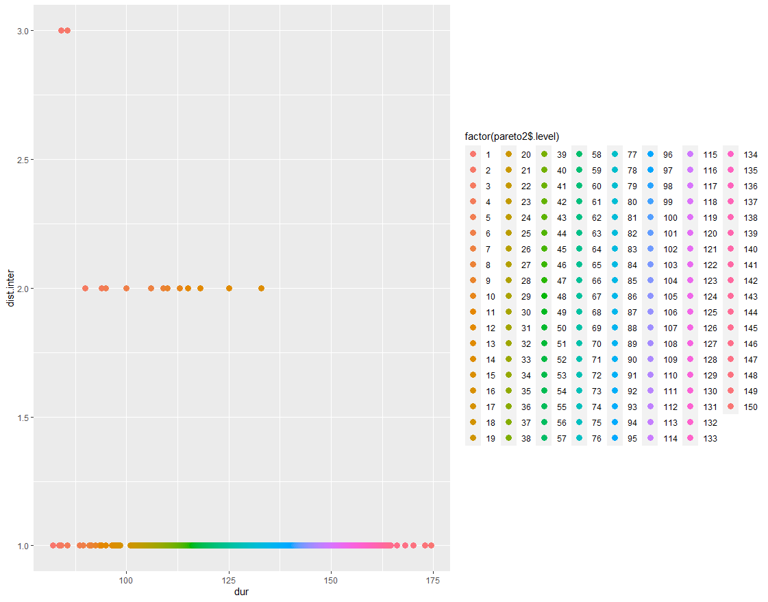
Fig 8 : Color Based Visualization of the alternatives
The figure above shows a graph displaying alternative combinations of the durations and distance between interruptions. They ranked based on the preference and 150 groups are presented here. As the low and high functions in our analysis affect each other. We can have graphical representation to understand how much sensitive change in one variable brings to the other one. For this, we will include the pareto frontier in our analysis.
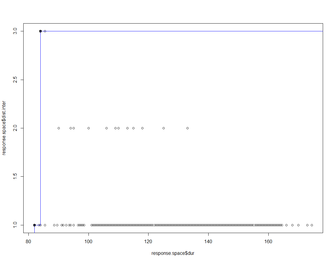
Fig 9 : Pareto Frontier Preference Ideal Combination
The blue lines present the pareto frontier and the black dots on them are the ideal combinations of the lifetime scenarios. Studying the plot, we can come to decision on the combination of duration and distance between the interruptions. This will be a trade-off from the ideal combination but we will attain a practical combination based on the resources we have and yet maintain the goal. On R-Studio, we could change our preference to high duration and low distance between interruption to compare results with the least favorable combination. This can help in ranking and decision making of the combinations.
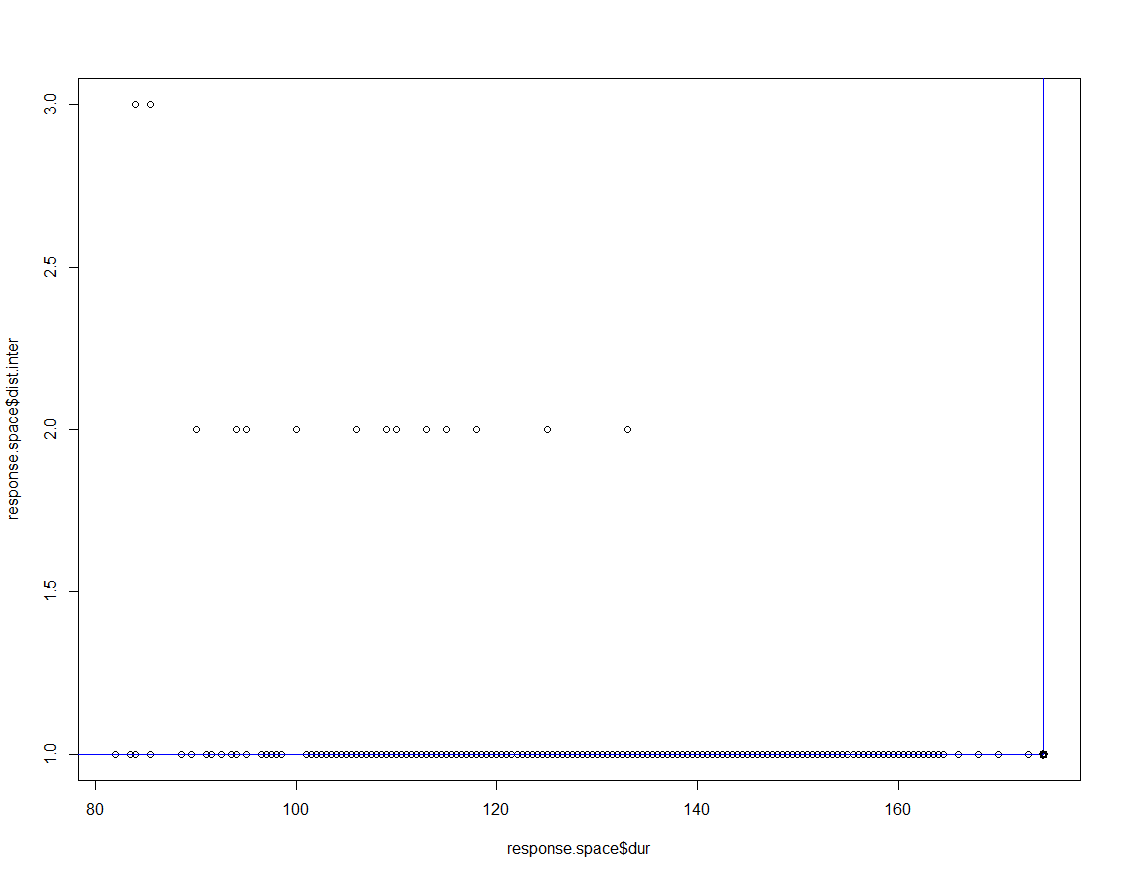
Fig 10 : Pareto Frontier Preference Worst Case