In the light of this analysis the need for optimization of different maintenance strategies and associated costs is imminent. In the following analysis, a large number of objective functions are optimized at the same time as to find the optimal solution to the underlying necessity to minimize costs of maintenance measures and maximize functionality time of the combined engineering systems.
As for the total number of interruptions and the maximum distance between interventions, we have taken into account a large set of variables that play a role in our analysis. The mean value of the duration between interventions is calculated to give a rough estimate about the total duration. The aim is to maximize this as the systems should be able to operate without interventions as much as possible.
As for the output variables the following have been added as variables: emission costs, maintenance costs and total costs. The upper and lower restrictions in maintenance time have been added to the function for each individual engineering product as well.
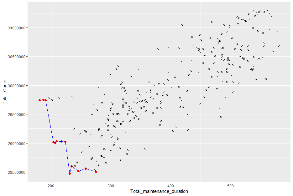
Given the above mentioned aims of maximizing time between interventions and limiting the total number of interventions and their duration, the results obtained have been displayed in a plot using the pareto-frontier as the optimal outcome between Total Costs and Total Maintenance Duration.
The number of optimal alternatives to look at has been increased to 200 and the generations to breed has been set to 10 to achieve optimal results. Of course, having this many possible outcomes, the computing and simulation time for this is especially high. Running the simulation again and changing the optimal number of alternatives to look at and also the number of generations to breed, we will get a slightly different plot as an outcome which is why the plot stated here should just be seen as an example of many possible optimal outcomes.
Pareto optimal state is achieved in this graph, meaning no further optimization of alternatives and scenarios is possible. All red marked points that can be seen connected by the blue line are optimal outcomes for a low cost and low maintenance duration scenario. The pareto frontier here aims to minimize both parameters for the x and y-axis.
Analyzing the first 5 points of the pareto frontier, it becomes clear that engineers will have to chose an optimal planning and maintenance strategy evaluating if the total maintenance factor is more important or the cost factor. Bearing in mind that costs are the main driver for multiple engineering projects, the pareto points have been structured showing the cheapest versions first.
Cheapest Maintenance Strategy:
Total Costs: 28.535.723 €
Total Duration: 267 days
Shortest Maintenance Strategy:
Total Costs: 29.498.706 €
Total Duration: 211 days
Observing the two optimal outcomes chosen here, the reduction of maintenance time by 56 days for all systems over the whole life span will result in an increase in maintenance costs for all systems by about 962.983 €. Maintenance planning engineers will have to choose the optimal strategy based on given conditions and requirements by the client and/or owner.
Increasing the total number of options showed within the graph, it is clear that there is a linear range of options that only becomes more costly and time consuming. Having set the population size to 200 and the generators to 20 has resulted in an optimal outcome as further research with higher numbers has shown. Higher numbers only result in a longer computing and calculating time and do not show better results for either maintenance time or costs.
Pareto Frontier showing the optimal solution
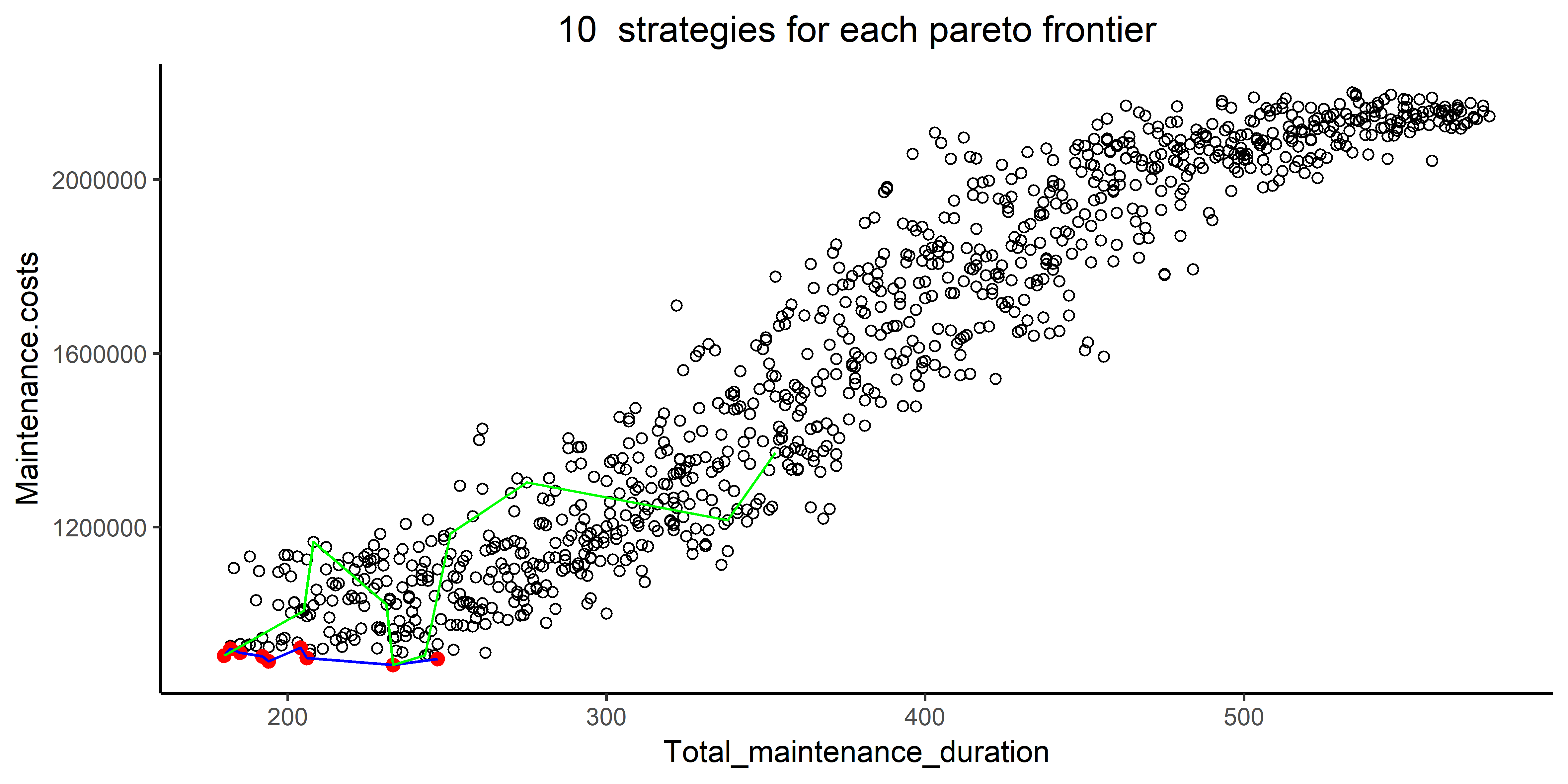
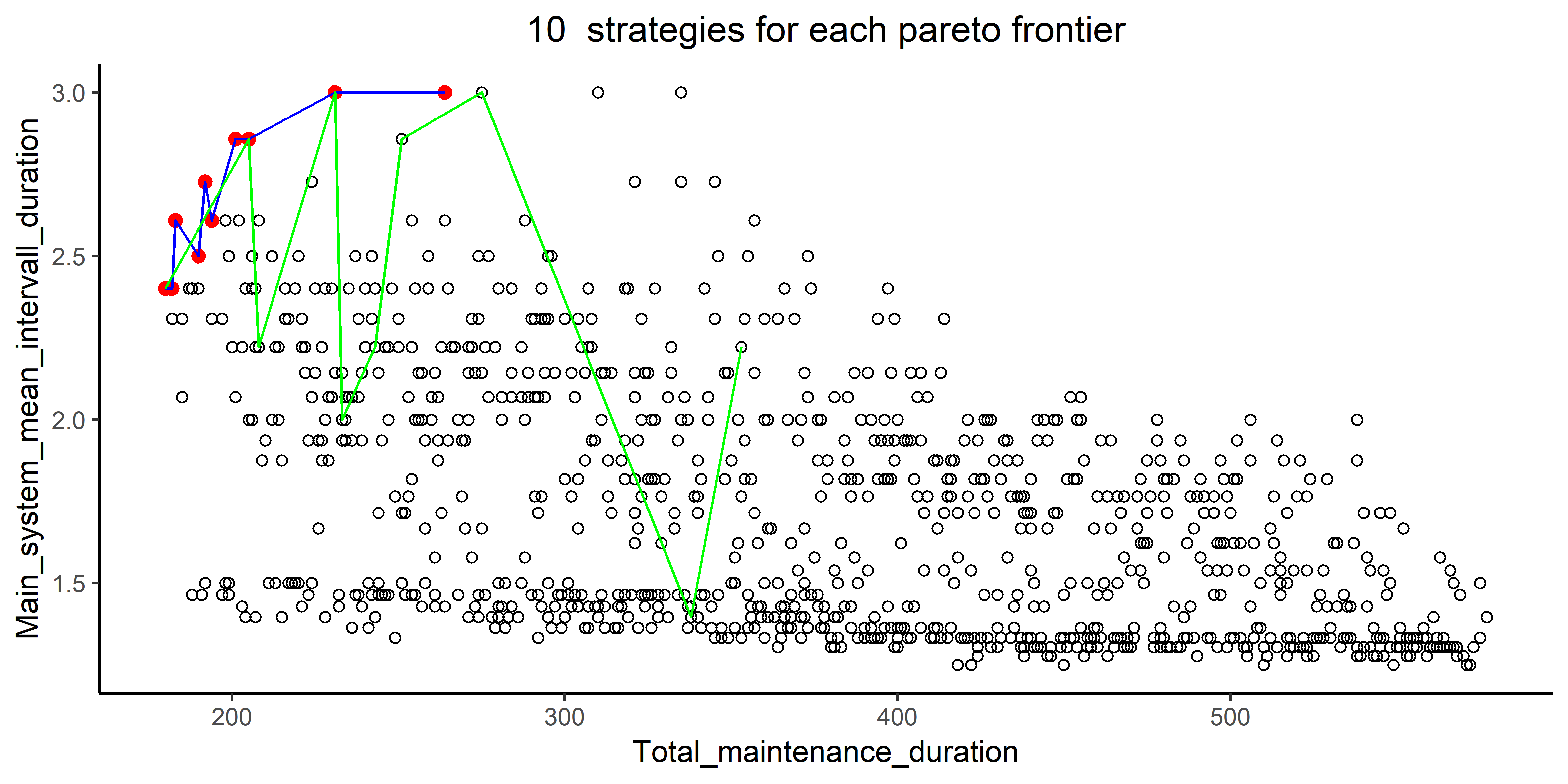
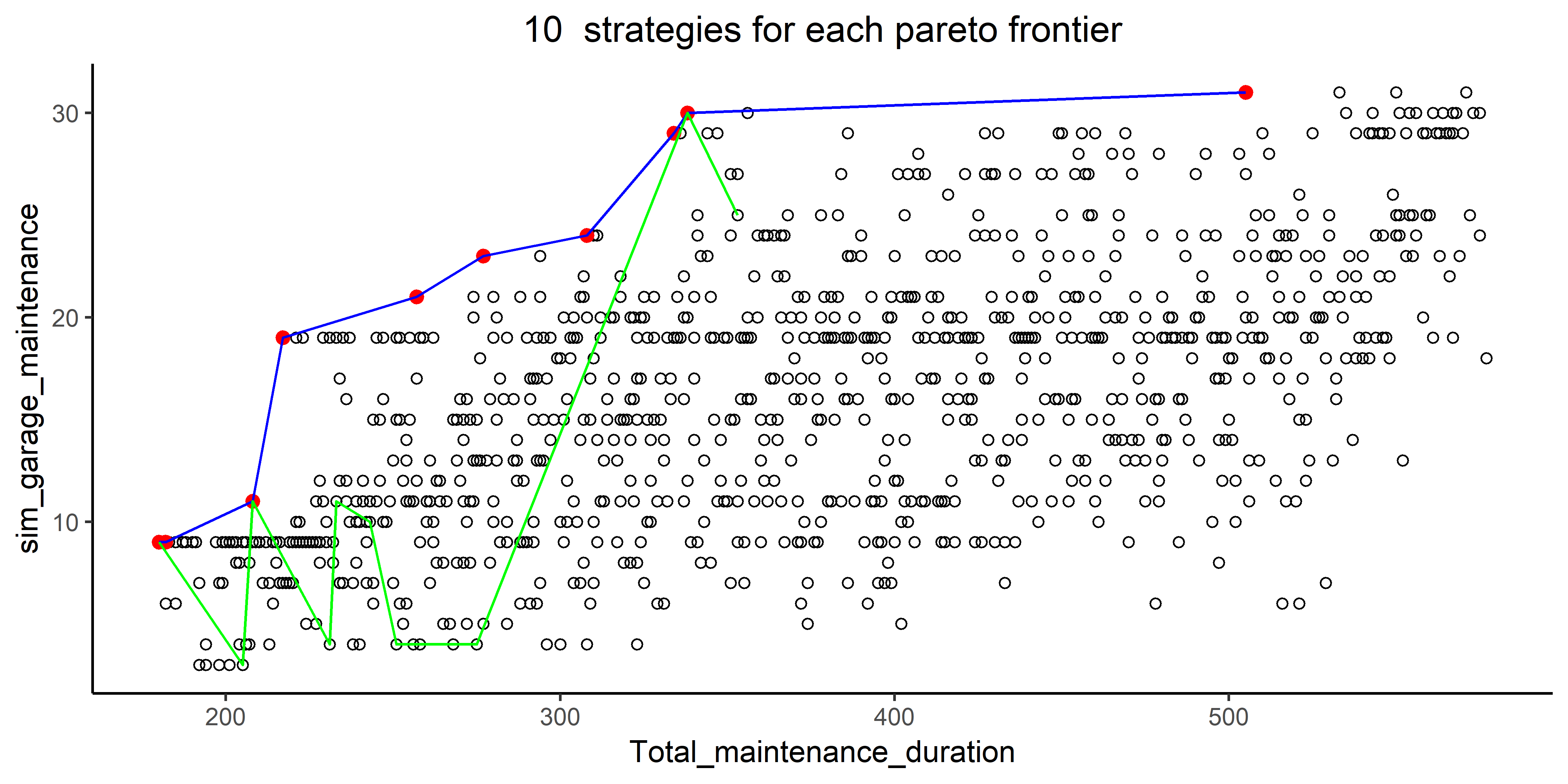
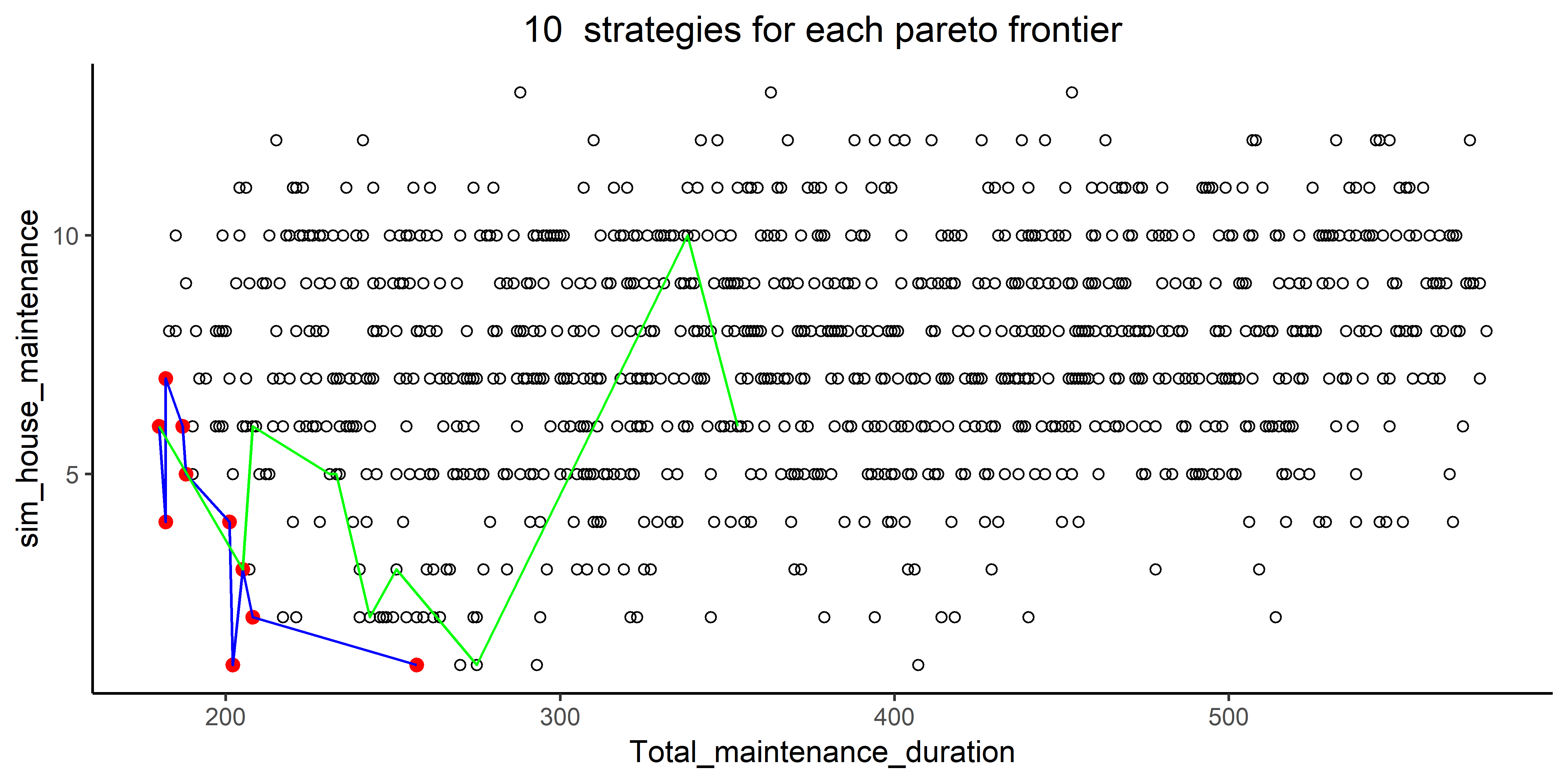
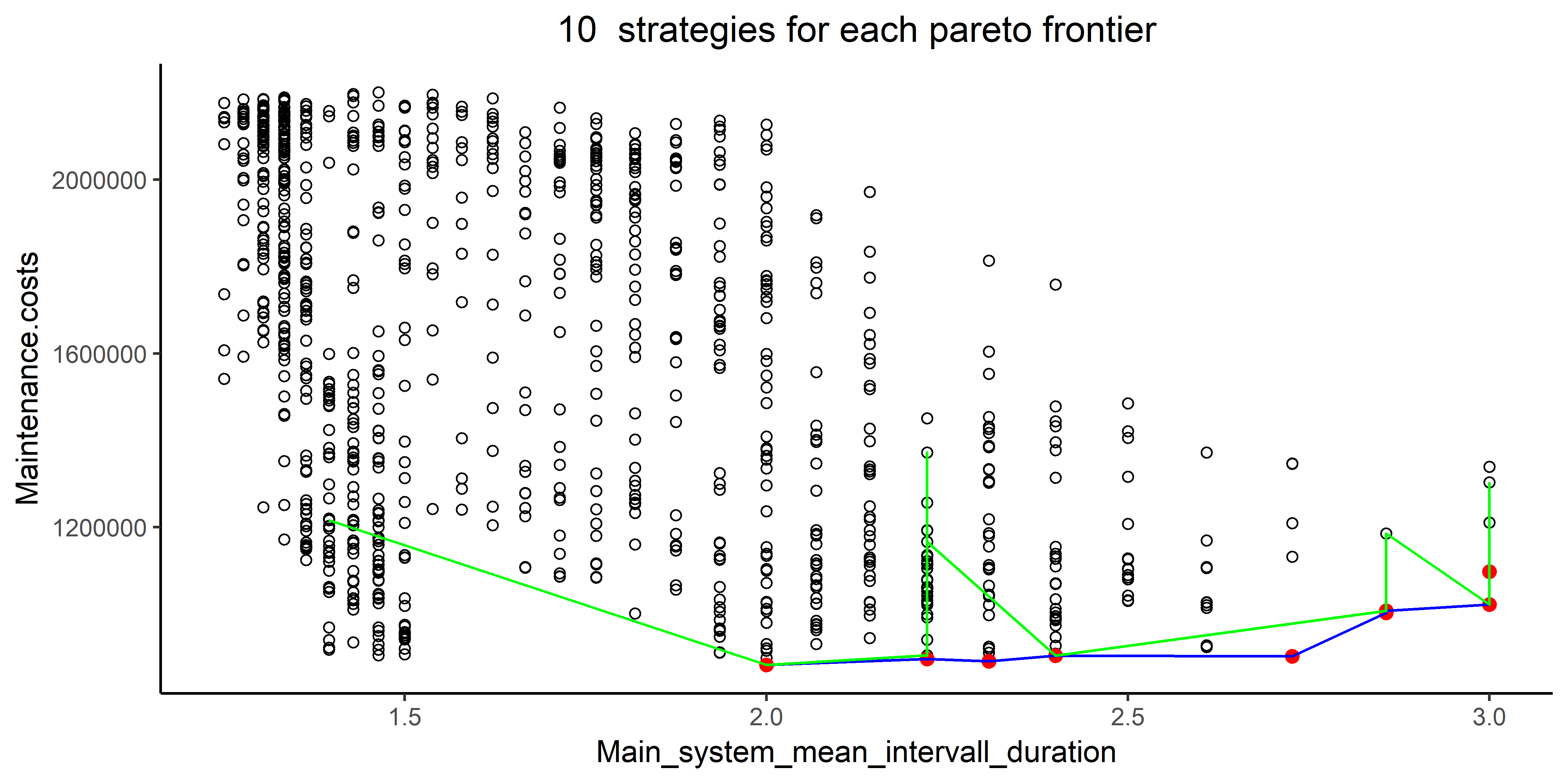
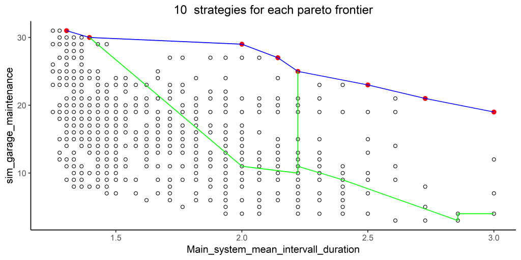
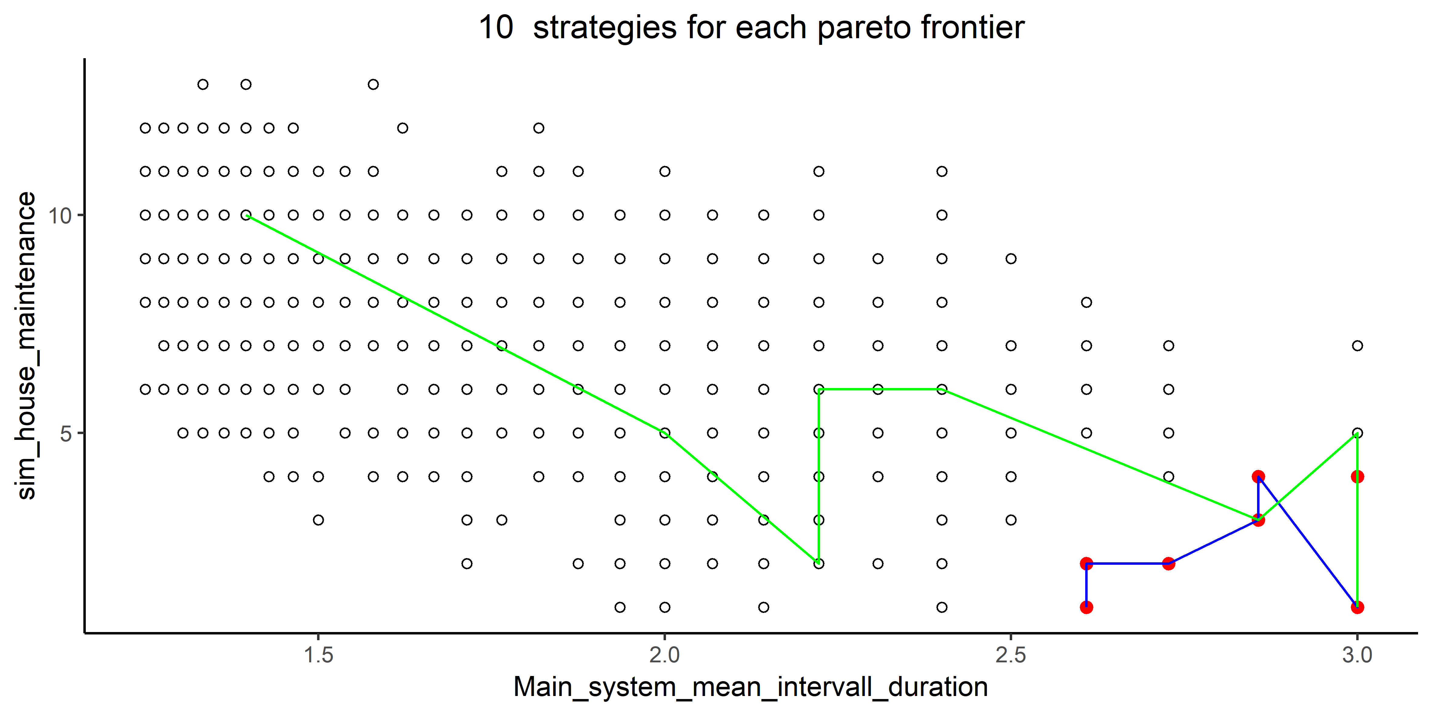
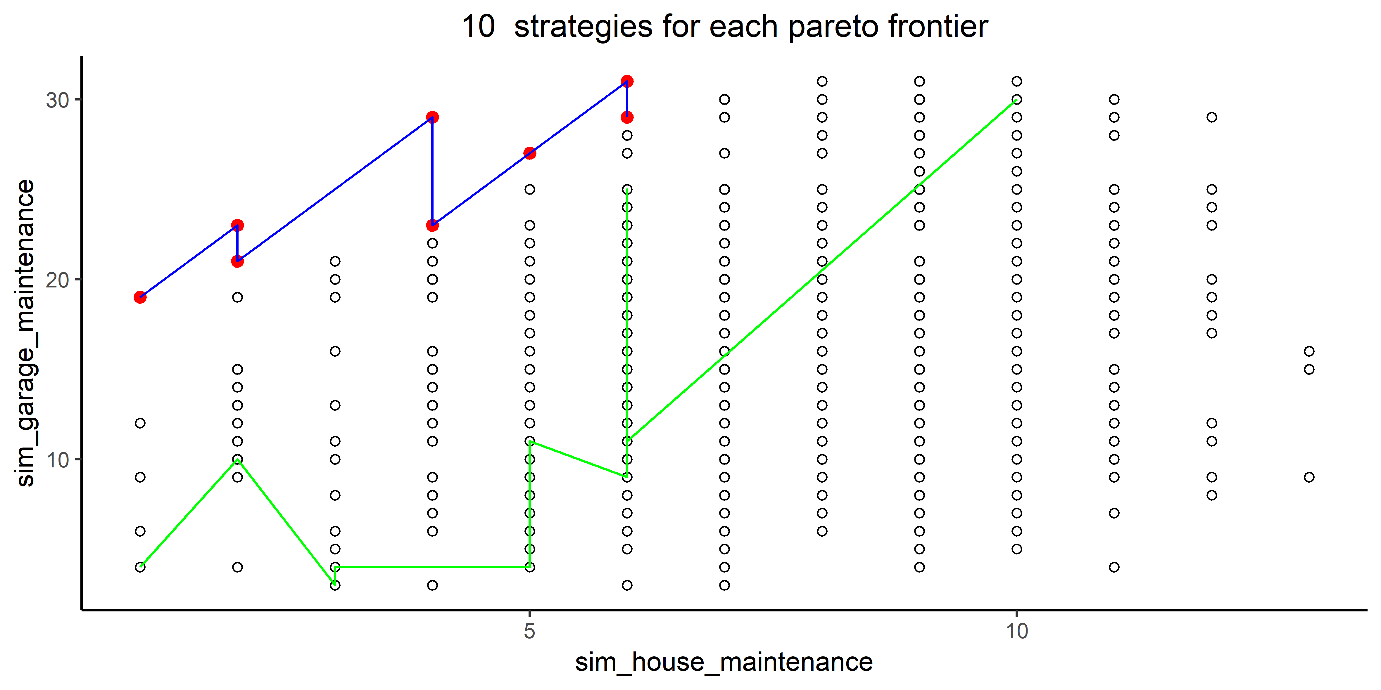
To show the different aspects of the multi objective optimization process of this model, all of the following five indicators were plotted out against each other: maintenance costs, total maintenance duration, main system mean interval time, simultaneous maintenance of the main system and the parking house/garage and the simultaneous maintenance of the main system and the residential house. The blue line with the red dots shows the pareto frontier if only the two indicators representing the axis are weighed against each other. The green line without dots show the absolute optimal pareto frontier for all five indicators with. In terms of programming, the green line is defined as:
pref.opt <- low(Total_maintenance_duration)* high(Main_system_mean_intervall) * low(Maintenance.costs) * low(sim_house_maintenance) * high(sim_garage_maintenance)
sky.pref.opt <- psel(r2Results.parallel, pref.opt, top = 10)
The data plotted in the following plots was derived using the model functions and a genetic algorithm (nsga2) with 20 generations and a population-size of 1000. In most plots one of the absolute optimal solutions is also the local optimal solution, which means, that despite having to optimize in regards to multiple objectives, some solutions can be actually satisfy most, if not all of the requirements.