With the multi-objective optimization approach, we combine the individual systems with each other by also combining their maintenance plans over 90 years of service life to balance objectives such as environmental impact, cost and social considerations. The main objectives for the optimized maintenance strategy are:
- Maximize the time between interventions.
- Minimize the time the system is not in use due to the interventions.
To this end, we have implemented a genetic algorithm for multi-objective optimization by defining the function, the number of input variables, the number of output actions and the lower and upper bounds for the input variables. The duration of the interventions for each system component is considered in the following specific range:
- Steel Purlins
- 1≤ IC ≤5
- 1≤ RP ≤10
- 30≤ PR ≤36
- 40≤ TR ≤60
- Beam and Slab
- 20≤ S ≤30
- 10≤ G ≤20
- 30≤ RS ≤40
- Railway Track
- 1≤ M ≤5
- 5≤ RPR ≤15
- 30≤ R ≤50
- Foundation
- 1≤ I ≤10
- 45≤ RC ≤55
- 75≤ RW ≤85
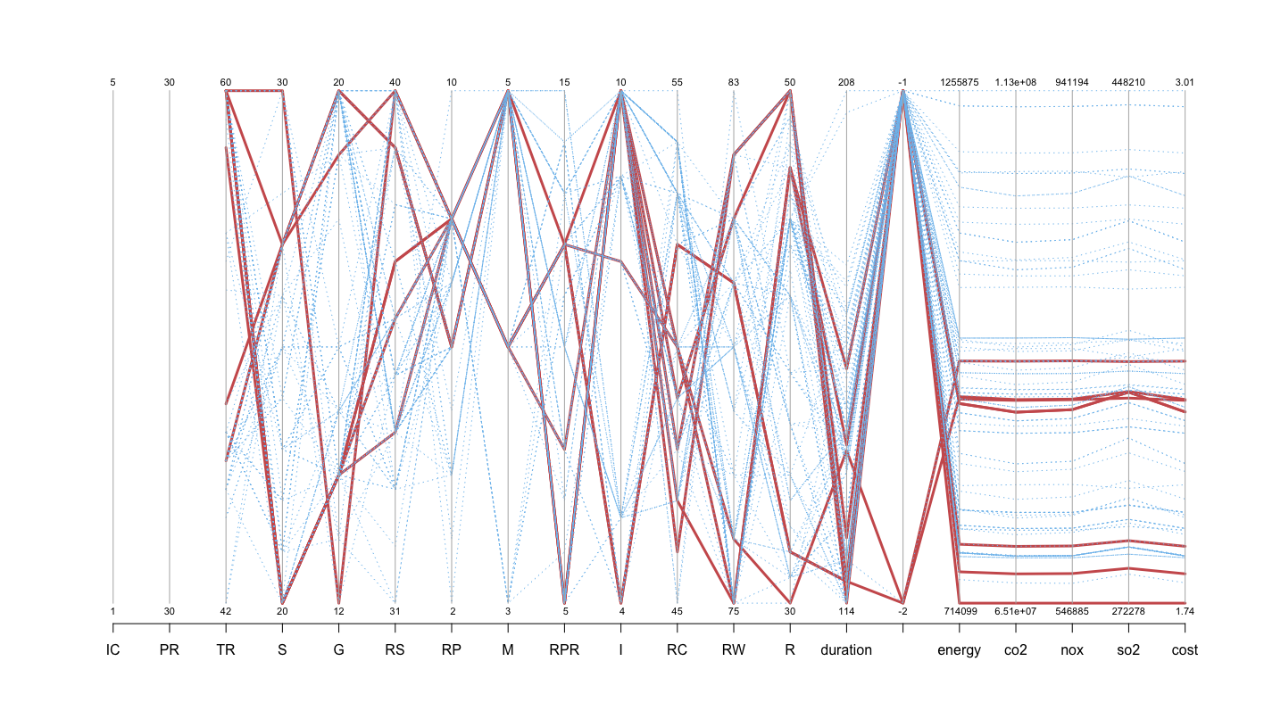
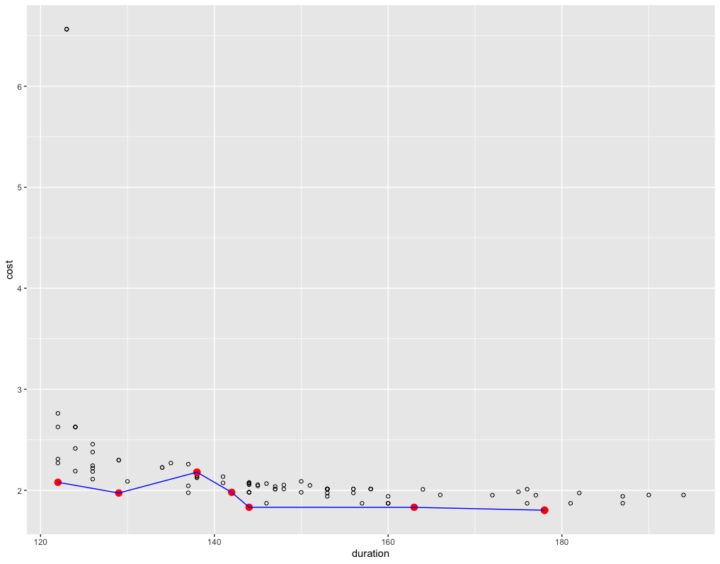
The results obtained were presented in a diagram using the Pareto frontier as the optimum result between total costs and total maintenance time:
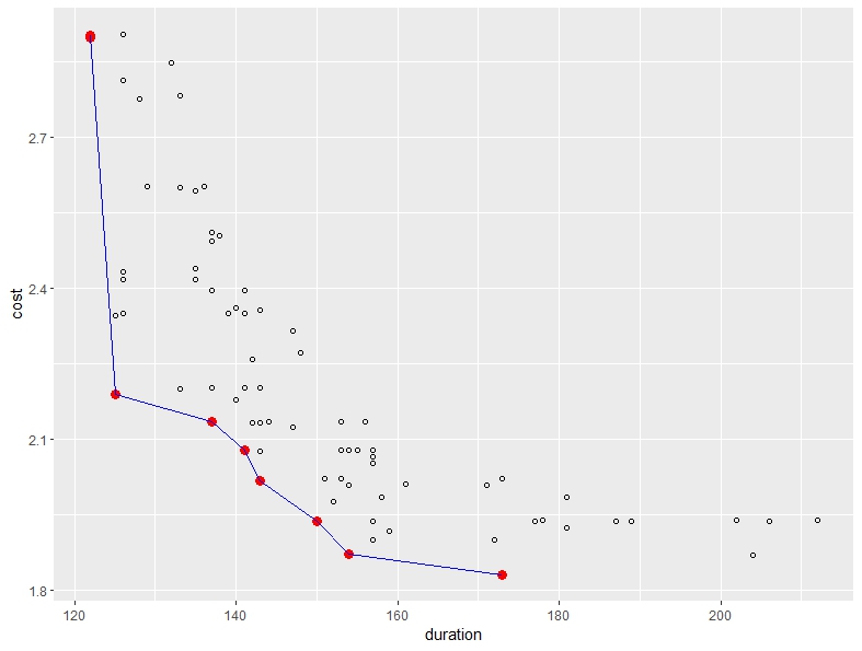
The first scenario created shows 8 different options for our performance criteria. It considers the time between interventions, the duration of the interventions and the cost of maintenance. If you run the simulation again and change the optimal number of alternatives to be considered and the number of generations to be produced, you get a slightly different diagram, which is why the diagram shown here should only be considered as an example of many possible optimal results.
The following figure illustrates the cumulative effects of the input parameters on the performance criteria. In this illustration, the red lines indicate optimal solutions, while the blue lines represent non-optimal solutions. It should be noted that the environmental costs remain relatively constant for all solutions, mainly due to emissions during construction. However, the optimal solutions show fluctuations for certain interventions. Differences in energy consumption and environmental costs between the solutions are evident, which may influence stakeholder decisions based on the objectives and priorities set.