2. Response space:
The number of possible combinations (maintenance strategies) included in the response space is calculated with the following equation:
r = n^3^5
r – the total number of the possible maintenance strategies
n – the amount of sampled maintenance intervals per individual intervention
s – the amount of the different interventions for each system
d – the number of the combined systems
So, in our case we calculated with n = 2, s = 3, d = 5, which leads to 32.768 different maintenance strategies. To generate the results the computer required about 11 minutes (Intel i5-6200u and 8GB DDR3 RAM). If the amount of sampled maintenance intervals was increased, the calculations would require too much time to complete this project. For if n = 3, the calculations would take about 80 hours and for n = 4 about 6007 hours, or in other words 250 days.
2.1. Maximum intervention time in the main system
Our main goal is to achieve the smallest possible duration time with the highest possible mean intervention time in the main system. As mentioned before, the maintenance of the house should not happen while the main system gets maintained due to high noise pollution whereas the maintenance of the garage should have a high overlap with the maintenance of the main system. Based on these objectives the best strategy was chosen.
If we look at Figure 3 it gives out one optimum combination. The exact combination is shown in Table 1 with a mean intervention time of 2.4 years (Figure 3). But within this strategy, we still have a high overlap of 3 to 7 years regarding the simultaneous repairs of the main system and the house.
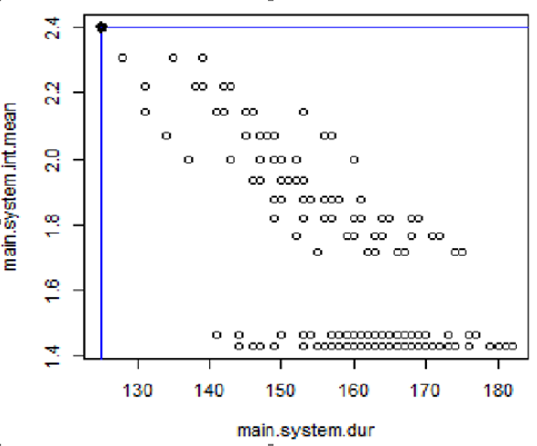
Figure 3: Pareto front shortest duration time of the main system, highest intervention time in the main system.
Table 1: duration strategy for the highest mean interventions, shortest duration time main system.
| Dam | Water supply | Tunnel | ||||||
| CF | GR | SL | PF | M | PR | PCR | CSR | CR |
| 11 | 22 | 22 | 3 | 11 | 53 | 3 | 18 | 54 |
To avoid the simultaneous maintenance of the main system and the house, we adjusted the strategy with a priority to minimize simultaneous repairs (Table 2: optimal combination of low simultaneous house maintenance with maintenance of the main system.Table 2). Applying this priority (low simultaneous house maintenance, low main system maintenance duration) we have a minimum overlap of simultaneous maintenance of 2 years (Figure 4). We also can see, that at this specific combination the main system duration is not at its minimum.
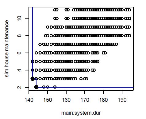
Figure 4: Pareto line of low simultaneous house maintenance and low main system duration.
The following Table 2 is showing the combination for minimized simultaneous repairs and the highest values for the mean intervention of the house and the main system.
Table 2: optimal combination of low simultaneous house maintenance with maintenance of the main system.
|
Dam |
Water supply |
Tunnel |
||||||
| CF | GR | SL | PF | M | PR | PCR | CSR | CR |
| 12 | 22 | 20 | 3 | 16 | 54 | 3 | 14 | 53 |
If we take a look at the optimal strategy for simultaneous maintenance of the garage and the main system, it is obvious that it is the same graph as in Figure 4 but with a mirrored pareto line (Figure 5). The graph also shows very clearly that with a longer duration in the main system, we also get more overlaps of simultaneous maintenance of the garage and the main system. We also can see that there are available combinations where the main system duration is as long as in Figure 4. Though the simultaneous repairs of garage and main system, as well as the time shifted repairs of the house and the main system are not at their optimum at those combinations.
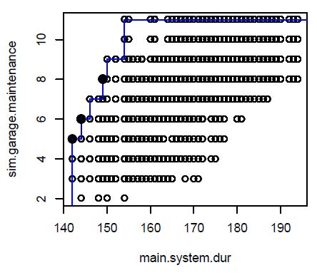
Figure 5: Pareto line for simultaneous garage and main system maintenance.
If we take a closer look at the optimal combination for a high overlap of the maintenance for the garage and the main system it stands out, that those are the same combinations for the dam, water supply system and the tunnel as in Table 2. Therefore, it must be a combination where both priorities (low simultaneous house maintenance with the main system and high simultaneous garage maintenance with the main system) are fulfilled. Though the duration time of all systems at this combinations is over 300 days. This makes sense because the single interventions should not overlay.
For the optimal maintenance just of the garage the following strategy is useful, high overlay:
Table 3: duration strategy for the longest simultaneous maintenance time of the garage and the main system.
|
Dam |
Water supply |
Tunnel |
Garage |
||||||||
| CF | GR | SL | PF | M | PR | PCR | CSR | CR | SDO | M | DR |
| 12 | 22 | 20 | 3 | 16 | 54 | 3 | 14 | 53 | 4 | 5 | 23 |
The strategy of the parking house maintenance is similar to the strategy of the house, this is reasonable because the strategy for the repair is contrary.
For the shortest duration time the intervention time is maximum with 2.4 years intervention time. In total the duration time for all systems is in a large interval between 260 d and 340 d.
As a conclusion if the mean intervention time is at its maximum the overlays with the maintenance of the house is at its minimum. If the mean intervention time is at its minimum, the simultaneous maintenance of the house could not reach the minimum of the overlay.
2.2. Minimum costs of the whole system
In the following we analyzed three different combinations with each other. The combination between all systems interventions mean, all systems duration and all systems costs. Additionally we formulated two conditions which are also shown in the analysis of the different combinations. In the first condition (red), we set a priority on short duration as well as low total costs. In the second condition (green) we took a closer look on the relation between the time distance between the single interventions and the total costs. Our aim here was again to find the combinations with a high temporal distance between the single interventions and low costs.
If we look at the graph for the combination of all systems interventions mean and all systems duration, we can get to the following conclusion: Short interventions are leading to long duration times in total, which is the condition of the red points. The opposite is shown by the green points, very long distances between the interventions are leading to a shorter duration time in total. Therefore it is clear that the distribution of the two formulated conditions (red and green) is not equally. Though we see an interval in the graph, where both conditions are more or less equally fulfilled (all system duration between 280 and 290; all systems intervention mean 1.8 and 1.9).
For the graph about all systems intervention mean and all systems costs we can make the following conclusions: Lower costs are directly linked with shorter time intervals between the interventions. Because the analyzed graph is equal to the second condition (green), the green points are forming the pareto line of the graph. If both conditions (red and green) should both be fulfilled the graph shows a possible interval between 1.7 and 1.9 for all systems intervention mean and 2.8 and 3 million Euros for all systems costs.
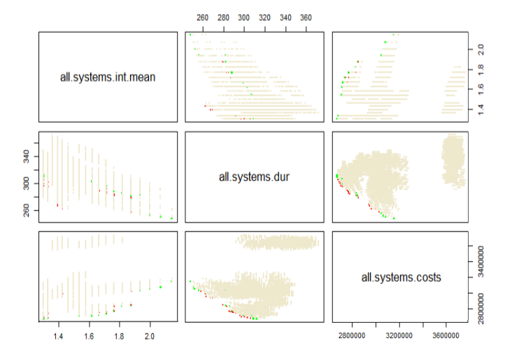
The following graph (Figure 7) shows the relation between the costs, the duration and the intervention time. It shows that the lowest price for the maintenance is not combined with the shortest duration time. Also the costs are raising if the time between the interventions is growing, but high intervention times are necessary for short duration times and low overlays for the simultaneous house maintenance. The opposite complied with the results of the simultaneous maintenance of the garage. As a result the cheapest combination would lead to a higher noise pollution for the house owners, because of the short time between the interventions.
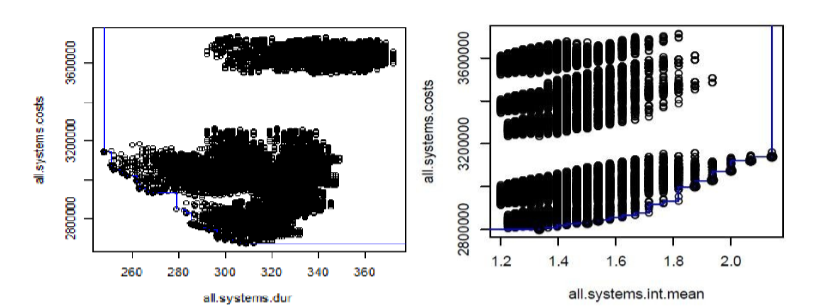
Figure 7: pareto line for all systems costs and all systems duration/all systems intervention mean.
2.3. Different duration strategies / iteration steps
So far we did our calculations with 2 variables out of the intervention interval. To optimize the results of the response space it is possible to increase the variable n for the calculation and use more variables out of the duration intervals. Due to the exponential growing of the respond space, the computational effort for solving the functions is increasing rapidly. To avoid long calculation times, it is also possible to adjust the duration intervals iteratively based on the results of the first calculation. On the other hand, it might be possible that the two randomly chosen numbers in the first iteration will not lead to the optimal duration strategies. Therefore certain solutions are excluded from the beginning on in this optimization strategy.
Because of the computing capacity we decide to adjust our intervals by ± 1 based on the first calculation.
Due to the results of our calculation, the shortest duration times for interventions of the main system leads to the following values for the subsystems. Starting with the dam, the values are:
Shortest duration main system (in total 125 days)
Table 4: duration strategy for the shortest duration time of the main system, first iteration.
| Dam | Water supply | Tunnel | House | Garage | ||||||||||
| CF | GR | SL | PF | M | PR | PCR | CSR | CR | M | PR | CR | SDO | M | DR |
| 12 | 21 | 21 | 3 | 17 | 50-52 | 3 | 16 | 51 | 13 | 17 | 52 | 4 | 5 | 23 |
Because the subsystem is not influencing the main system, duration times of the subsystem can be neglected.House / Garage: vary widely
As mentioned, before we restricted the ranges of the intervention intervals in relation to the upper results from Table 4. Just the results of the main system have been optimized, due to vary widely ranges of the subsystem.
In the second iteration step, the values for the maintenance strategy is shown below (Table 5) and it is obvious that we have an improvement of the duration time about 12% (from 125 days down to 111 days). To optimization takes place in the intervention interval for the pipe replacement in the drinking water system (from 52 to 51 years) and in the Concrete and steel replacement – CSR (from 16 up to 17).
This kind of iterative optimization can also be applied on any other priority/case.
Table 5: duration strategy for the shortest duration time of the main system, second iteration.
| Dam | Water supply | Tunnel | ||||||
| CF | GR | SL | PF | M | PR | PCR | CSR | CR |
| 12 | 21 | 21 | 3 | 17 | 51 | 3 | 17 | 51 |
Lowest costs in totalHouse / Garage: vary widely
In the next tables (Table 6, Table 7) the optimization process was aimed at the lowest costs in total for the whole system. So, in Table 6 the results of the first iteration are shown and like above, in Table 7 the results of the adjusted values are presented.
Table 6: duration strategy for the lowest costs for the maintenance of the main system, first iteration.
| Dam | Water supply | Tunnel | House | Garage | ||||||||||
| CF | GR | SL | PF | M | PR | PCR | CSR | CR | M | PR | CR | SDO | M | DR |
| 12 | 21 | 21 | 2-3 | 17 | 50-52 | 2-3 | 16 | 51 o 55 | high variation | 5 | 6 | 25 | ||
Table 7:duration strategy for the lowest costs for the maintenance of the main system, second iteration.
| Dam | Water supply | Tunnel | House | Garage | ||||||||||
| CF | GR | SL | PF | M | PR | PCR | CSR | CR | M | PR | CR | SDO | M | DR |
| 12 | 20 | 20 | 2 | 16 | 53 | 3 | 15 | 54 | high variation | 6 | 7 | 24 | ||
Apparently the values in most of the cases decrease. This could be caused by the mathematical function behind the calculation of the total costs because every year the costs for a postponed intervention is raising 10 %. The deck replacement for the garage, for example is the most expensive intervention in the whole system. Caused by the cost increase, the deck replacement in the garage starts a year earlier than in the first calculation. This leads to a cost reduction round about 50.000 €.v.w. – vary widely